Genie 系列技术演进
最后更新: 2026-04-14 | 深度调研
Genie 1 整体架构图(原论文 arXiv:2402.15391 Figure 2)
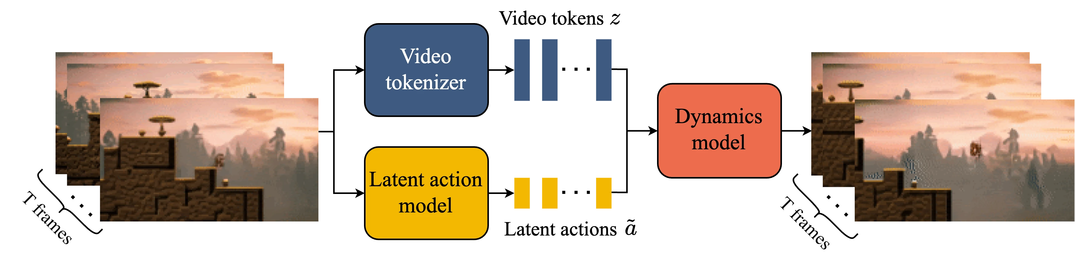
Genie 1 (2024.02) — 10.7B参数
-
ST-ViViT视频分词器(200M): VQ-VAE+时空因子化Transformer, codebook 1024
-
潜在动作模型LAM(300M): 无监督动作学习核心创新, 8个离散动作code
-
ST-maskGIT动力学模型(10.1B): 解码器only MaskGIT+ST-Blocks
-
训练: 680万片段(3万小时), 256 TPUv5p, 942B tokens
-
局限: 1 FPS, 160x90分辨率
Genie 2 (2024.12) — 3D世界
-
自回归潜在扩散模型, 单图→可交互3D世界
-
世界一致性约1分钟, 分辨率约360p
-
涌现: 角色动画/物理/NPC行为/多视角
-
未公开技术论文(仅博客)
Genie 3 (2025.08) — 实时720p
-
首个实时交互通用世界模型: 20-24 FPS, 720p
-
四组件: 视觉分词器+动力学模型+动作接口+渲染器
-
隐式物理学习(无硬编码引擎)
-
记忆: 最长1分钟回溯窗口
-
训练: 30000+小时游戏视频+网络视频
GameNGen vs DIAMOND vs Oasis vs Genie
-
GameNGen: SD v1.4改造, 860M, DOOM专用, PSNR 29.43
-
DIAMOND: EDM U-Net, 4.4M(Atari)/381M(CSGO), n=3去噪步
-
Oasis: DiT扩散, 500M, Minecraft, Diffusion Forcing
-
Genie 3: 自回归, 最强通用性, 720p实时
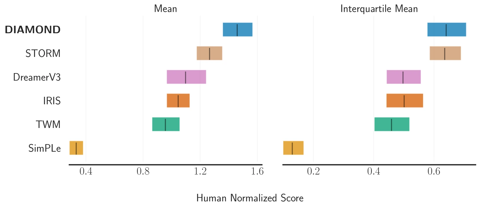
DIAMOND Atari-100k 性能对比图(arXiv:2405.12399 Figure 1)
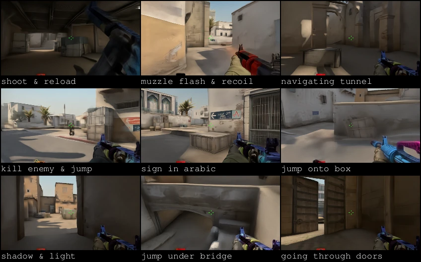
DIAMOND CS:GO 世界模型生成效果(arXiv:2405.12399 Figure 6)
参考
工程实现细节
Genie LAM(潜在动作模型)信息瓶颈实现
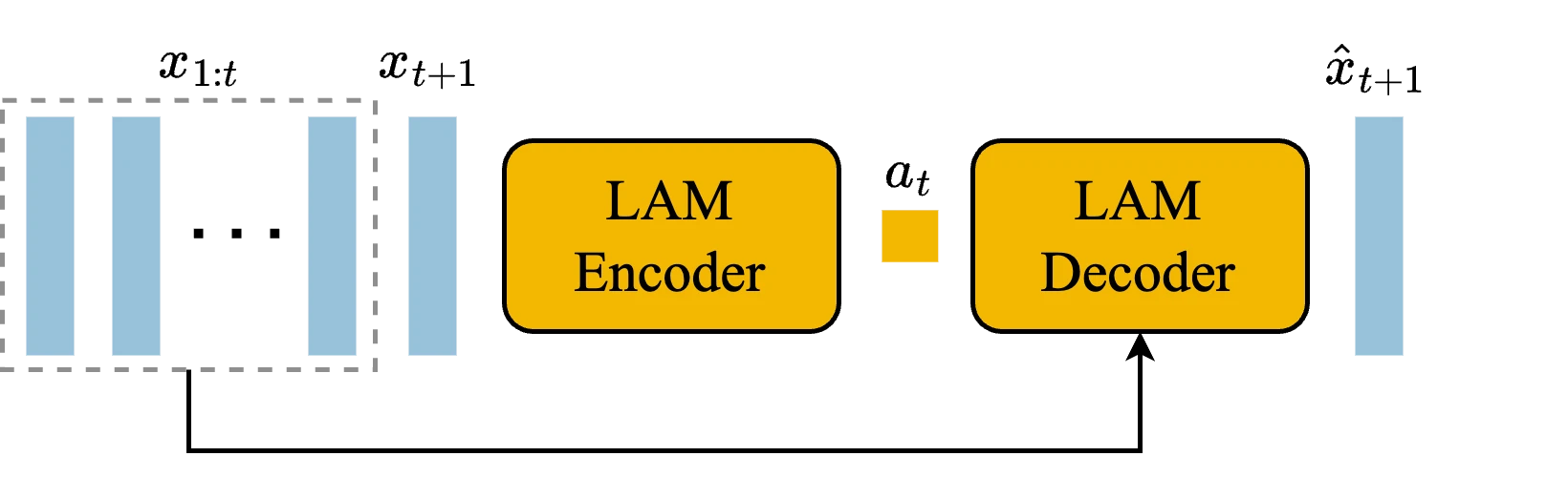
核心创新:从无标签视频自动学习离散动作。诀窍是"非对称信息"——编码器能看到下一帧,但解码器只能用历史+动作重建下一帧,这迫使动作向量编码有意义的变化。
import torch
import torch.nn as nn
import torch.nn.functional as F

class LatentActionModel(nn.Module):
    """
    Genie 1 LAM: 300M 参数, 20 层, d=1024, 16 heads, patch=16

    关键设计:
    - Encoder 能看到 (x_1..x_t, x_{t+1})  — 历史 + 下一帧
    - Decoder 只能看到 (x_1..x_t, a_t)    — 历史 + 学到的动作
    - 这个信息不对称是动作学习的根本
    """
    def __init__(self, d_model=1024, n_layers=20, codebook_size=8, d_latent=32):
        super().__init__()

        # Patch=16 (比 ST-ViViT 的 patch=4 更大)
        # 对于 160×90 视频: 160/16 × 90/16 ≈ 10 × 5 = 50 patches/frame
        self.patch_embed = nn.Conv2d(3, d_model, kernel_size=16, stride=16)

        # Encoder: 20 层 Transformer, 同时看历史+下一帧
        self.encoder = nn.ModuleList([
            TransformerBlock(d_model, n_heads=16) for _ in range(n_layers)
        ])
        self.to_action = nn.Linear(d_model, d_latent)  # 投影到潜动作空间

        # VQ codebook: 8 个离散动作
        self.codebook = nn.Embedding(codebook_size, d_latent)
        self.codebook_size = codebook_size

        # Decoder: 只接收历史 + 离散动作
        # ST-ViViT Tokenizer 是独立的 (200M), 这里假设外部处理
        self.decoder = STMaskGITDecoder(d_model=1024)

    def forward(self, frames):
        """
        frames: (B, T+1, C, H, W)  — T 历史帧 + 1 下一帧
        返回: (frame_tokens_pred, action_indices)
        """
        B, T1, C, H, W = frames.shape
        T = T1 - 1

        # ========== 1. Encoder: 看全部 T+1 帧 ==========
        # Patch 化
        patches = self.patch_embed(frames.flatten(0, 1))       # (B*(T+1), D, h/16, w/16)
        patches = patches.flatten(2).transpose(1, 2)           # (B*(T+1), n_patches, D)
        patches = patches.reshape(B, T1 * n_patches, d_model)

        # 时序+空间位置编码
        patches = patches + self.pos_embed

        # 20 层 Transformer
        for blk in self.encoder:
            patches = blk(patches)                             # (B, (T+1)*n_patches, D)

        # 取最后一帧的聚合表示 (e.g., 平均池化)
        last_frame_repr = patches[:, -n_patches:].mean(dim=1)  # (B, D)

        # ========== 2. 投影到 32-dim 潜动作空间 ==========
        latent_action = self.to_action(last_frame_repr)        # (B, 32)

        # ========== 3. VQ 量化到 8 个离散 code ==========
        # 距离计算
        distances = torch.cdist(
            latent_action.unsqueeze(1),                        # (B, 1, 32)
            self.codebook.weight.unsqueeze(0)                  # (1, 8, 32)
        ).squeeze(1)                                           # (B, 8)
        action_idx = distances.argmin(dim=-1)                  # (B,)

        # 直通估计器 (STE)
        a_quantized = self.codebook(action_idx)                # (B, 32)
        a_quantized = latent_action + (a_quantized - latent_action).detach()

        # ========== 4. Decoder: 仅用 (历史帧, a_t) 重建下一帧 ==========
        history_frames = frames[:, :T]                         # (B, T, C, H, W)
        next_frame_logits = self.decoder(history_frames, a_quantized)

        # 损失: 重建下一帧的 token logits (cross-entropy)
        # next_frame 被 ST-ViViT 编码成 token, 作为目标
        target_tokens = st_vivit.encode(frames[:, T])          # (B, n_patches)
        L_recon = F.cross_entropy(
            next_frame_logits.reshape(-1, vocab_size),
            target_tokens.reshape(-1)
        )

        # VQ 损失
        L_codebook = F.mse_loss(a_quantized.detach(), latent_action)
        L_commit = F.mse_loss(a_quantized, latent_action.detach())

        L_total = L_recon + L_codebook + 0.25 * L_commit
        return L_total, action_idx

# ============ 为什么信息瓶颈强制动作学习 ============
# 如果 Decoder 能看到下一帧 → LAM 只需输出恒等映射, 动作无意义
# 但 Decoder 只能看到 (历史, 动作) → 动作必须编码 "从历史到下一帧的变化"
# codebook_size=8 进一步限制 → 只能编码 8 种最重要的变化模式
#   → 跑/跳/左/右/攻击/...等游戏动作自然涌现
ST-maskGIT 动力学模型(10.1B)
Genie 1 LAM 架构图(原论文 Figure 5)
class STMaskGITDynamics(nn.Module):
    """
    Genie 1 动力学模型: Decoder-only MaskGIT + ST-Blocks
    输入: 历史视频 tokens + 动作 token
    输出: 下一帧的 tokens (MaskGIT 并行预测)
    """
    def __init__(self, n_layers=48, d_model=2048, codebook=1024):
        super().__init__()
        self.st_blocks = nn.ModuleList([STBlock(d_model) for _ in range(n_layers)])
        self.output_head = nn.Linear(d_model, codebook)

    def forward(self, tokens_history, action_token, mask_ratio):
        """
        tokens_history: (B, T*n_patches) 过去帧的 tokens
        action_token: (B, 1) 离散动作
        mask_ratio: 随机 mask 下一帧一部分 tokens 让模型预测

        训练: BERT 式掩码预测
        """
        # 构建 input 序列: [history_tokens | action | masked_next_tokens]
        # 以 cosine schedule 随机 mask 部分下一帧 tokens
        next_tokens_masked = apply_mask(target_tokens, mask_ratio)

        seq = torch.cat([
            embed(tokens_history),
            embed(action_token),
            embed(next_tokens_masked)
        ], dim=1)

        # 因果掩码: 下一帧内部可互相看, 但只能看过去不看未来
        for blk in self.st_blocks:
            seq = blk(seq)

        logits = self.output_head(seq[:, -n_patches:])  # 只预测被 mask 部分
        return logits

class STBlock(nn.Module):
    """
    Spatiotemporal Block: 分离空间 + 时间注意力
    """
    def __init__(self, d_model):
        super().__init__()
        self.spatial_attn = nn.MultiheadAttention(d_model, 16, batch_first=True)
        self.temporal_attn = nn.MultiheadAttention(d_model, 16, batch_first=True)
        self.mlp = MLP(d_model)

    def forward(self, x):
        # x: (B, T, N_spatial, D)
        B, T, N, D = x.shape

        # Spatial attention: 帧内 token 之间 (B*T, N, D)
        x_sp = x.reshape(B*T, N, D)
        x_sp = x_sp + self.spatial_attn(x_sp, x_sp, x_sp)[0]

        # Temporal attention: 跨帧同 token (B*N, T, D)
        x_tp = x_sp.reshape(B, T, N, D).transpose(1, 2).reshape(B*N, T, D)
        x_tp = x_tp + self.temporal_attn(x_tp, x_tp, x_tp)[0]

        # MLP
        x = x_tp.reshape(B, N, T, D).transpose(1, 2)
        x = x + self.mlp(x)
        return x

# ============ MaskGIT Cosine Schedule Inference ============
def maskgit_sample(model, history, action, n_steps=8):
    """
    MaskGIT 非自回归并行采样
    """
    B, N = history.shape[0], n_patches  # 下一帧要生成 N 个 tokens
    next_tokens = torch.full((B, N), MASK_TOKEN_ID)  # 全部 masked

    for step in range(n_steps):
        logits = model(history, action, next_tokens)  # (B, N, vocab)
        probs = F.softmax(logits, dim=-1)
        sampled = probs.argmax(dim=-1)                # (B, N)

        # Cosine schedule: 每步保留 (1 - cos(π * (step+1)/n_steps)/2) 的 token
        keep_ratio = 1 - (1 + np.cos(np.pi * (step+1) / n_steps)) / 2
        n_keep = int(N * keep_ratio)

        # 保留最高置信度的 n_keep 个 token, 其余重新 mask
        confidence = probs.gather(-1, sampled.unsqueeze(-1)).squeeze(-1)  # (B, N)
        top_idx = confidence.topk(n_keep, dim=-1).indices
        keep_mask = torch.zeros_like(next_tokens, dtype=bool)
        keep_mask.scatter_(1, top_idx, True)

        next_tokens = torch.where(keep_mask, sampled, torch.full_like(sampled, MASK_TOKEN_ID))

    return next_tokens
GAIA-2 双峰时间采样与多视角一致性
# ============ 双峰 Logit-Normal 时间采样 ============
def sample_time_bimodal(batch_size):
    """
    GAIA-2 训练时的 τ 采样 (Flow Matching 时间)

    双峰设计的 motivation:
    - 主峰 μ=0.5, σ=1.4, p=0.8: 覆盖中段去噪, 网络学习主要降噪能力
    - 次峰 μ=-3.0, σ=1.0, p=0.2: 重点训练近纯噪声情况 (τ 接近 0)
                                 这里网络需要学会从噪声生成大结构

    为什么是 logit-normal 而非 uniform:
    - 均匀分布在极端 τ 处梯度不稳定 (尺度巨大差异)
    - Logit-Normal 在 sigmoid 变换后给特定区域更高采样密度
    """
    use_secondary = torch.rand(batch_size) < 0.2  # 20% 概率用次峰

    # 主峰
    z_main = torch.randn(batch_size) * 1.4 + 0.5
    # 次峰
    z_sec = torch.randn(batch_size) * 1.0 - 3.0

    z = torch.where(use_secondary, z_sec, z_main)
    tau = torch.sigmoid(z)  # 映射到 [0, 1]
    return tau

# ============ 相机几何位置编码 ============
class CameraAwarePositionalEncoding(nn.Module):
    """
    GAIA-2 多视角注意力: 5 摄像头各自位置编码
    包含: 空间正弦编码 + 相机内参 + 相机外参 + 畸变
    """
    def __init__(self, d_model=4096):
        super().__init__()
        self.d_model = d_model
        # 几何参数投影到 d_model
        self.cam_param_proj = nn.Linear(16, d_model)  # 4 intrinsic + 4 quat + 3 trans + 5 dist = 16

    def encode_camera(self, intrinsics, extrinsics_R, extrinsics_T, distortion):
        """
        intrinsics: (B, 4) [fx, fy, cx, cy] 归一化后
        extrinsics_R: (B, 3, 3) 旋转矩阵
        extrinsics_T: (B, 3) 平移
        distortion: (B, 5) 径向+切向畸变系数
        """
        B = intrinsics.shape[0]
        # 旋转 → 四元数 (连续, 4-D)
        quat = rotation_to_quaternion(extrinsics_R)    # (B, 4)

        # 拼接所有几何参数
        geom = torch.cat([
            intrinsics,      # (B, 4)
            quat,            # (B, 4)
            extrinsics_T,    # (B, 3)
            distortion,      # (B, 5)
        ], dim=-1)           # (B, 16)

        cam_embed = self.cam_param_proj(geom)          # (B, d_model)
        return cam_embed

    def forward(self, patch_tokens, camera_params, patch_positions_2d):
        """
        patch_tokens: (B, N_cameras  H  W, D)  5 摄像头的 patch tokens
        camera_params: dict per camera
        patch_positions_2d: (N, 2) 每 patch 的 (row, col)
        """
        B, N, D = patch_tokens.shape

        # 2D 正弦位置编码
        pos_enc = sinusoidal_2d(patch_positions_2d, D)  # (N, D)

        # 每 patch 所属的相机编码
        cam_per_patch = camera_assignment(patch_positions_2d)  # (N,) camera idx
        cam_embed_per_patch = cam_embed[cam_per_patch]         # (N, D)

        return patch_tokens + pos_enc.unsqueeze(0) + cam_embed_per_patch.unsqueeze(0)

# ============ 多视角联合注意力 ============
def multi_view_attention(tokens_all_cameras):
    """
    tokens_all_cameras: (B, 5HW, D) - 5 摄像头拼接后的 tokens
    这里的 Attention 天然跨视角 — 每个 token 可以 attend 任何其他 token
    但位置编码告诉它哪些 token 来自哪个相机 (几何感知)
    """
    # 相机间几何关系通过位置编码隐式编码
    # 不需要特殊的 cross-view attention 模块
    return transformer(tokens_all_cameras)
GAIA-2 自车动态 Symlog + AdaLN 注入
def symlog_transform(x):
    """
    对称对数变换: 处理有符号数值 (速度、曲率)
    symlog(x) = sign(x) * log(|x| + 1)
    关键性质: 对称性保留方向信息, 压缩极端值

    应用例子:
      velocity_m_per_s ∈ [-30, +30] → symlog ∈ [-3.4, +3.4]
      curvature ∈ [-0.1, +0.1] → symlog ≈ [-0.095, +0.095]
    """
    return torch.sign(x) * torch.log(torch.abs(x) + 1)

class EgoDynamicsAdaLN(nn.Module):
    """
    自车动态 (速度, 曲率) 通过 AdaLN 注入 DiT block
    不同于文本条件(交叉注意力),动态量直接调制 LN 参数
    """
    def __init__(self, d_model=4096):
        super().__init__()
        # symlog(speed) + symlog(curvature) + time_embed → MLP → (γ, β)
        self.ego_encoder = nn.Sequential(
            nn.Linear(3, 128),      # [speed, curvature, time_tau]
            nn.SiLU(),
            nn.Linear(128, d_model * 2)  # 输出 γ, β
        )

    def forward(self, x, ego_state, tau):
        """
        x: (B, N, D) — DiT 中间特征
        ego_state: (B, 2) — [speed, curvature]
        tau: (B,) — Flow Matching 时间
        """
        # 1. Symlog 变换让大小值对称
        symlog_speed = symlog_transform(ego_state[:, 0:1])
        symlog_curv = symlog_transform(ego_state[:, 1:2])
        tau_emb = sinusoidal_encoding(tau)  # (B, ?)

        # 2. 拼接并编码
        cond = torch.cat([symlog_speed, symlog_curv, tau_emb], dim=-1)
        gamma_beta = self.ego_encoder(cond)  # (B, 2*D)
        gamma, beta = gamma_beta.chunk(2, dim=-1)  # 各 (B, D)

        # 3. AdaLN: γ * LN(x) + β
        x_norm = F.layer_norm(x, x.shape[-1:])
        return x_norm * (1 + gamma.unsqueeze(1)) + beta.unsqueeze(1)
DIAMOND EDM: n=3 步去噪如何实现
# DIAMOND 基于 EDM 框架, 仅需 n=3 步即可生成高质量下一帧
# 这比 DDPM (~50 步) / Sora (~30步) 快得多

class DIAMONDDenoiser(nn.Module):
    """
    U-Net 2D with Adaptive Group Norm for action conditioning
    CS:GO: 381M 参数; Atari: 仅 4.4M 参数
    """
    def __init__(self, action_dim=17):  # CS:GO: 鼠标 XY + 15 按键
        super().__init__()
        self.unet = UNet2D(base_channels=128)  # Atari 小; CS:GO 大
        # 动作 → scale/shift (per GN group)
        self.action_encoder = nn.Linear(action_dim, 2 * 32)  # 32 groups

    def forward(self, x_noisy, sigma, past_frames, action):
        """
        x_noisy: (B, C, H, W) — 带噪的下一帧
        sigma: (B,) — 噪声水平 (EDM 用 σ 而非 t)
        past_frames: (B, C*n_past, H, W) — 过去 n 帧沿通道拼接
        action: (B, action_dim)
        """
        # EDM 预条件化
        c_in = 1 / torch.sqrt(sigma2 + 0.52)    # 归一化输入
        c_noise = sigma.log() / 4
        c_skip = 0.52 / (sigma2 + 0.52)
        c_out = sigma * 0.5 / torch.sqrt(sigma2 + 0.52)

        # 输入: 预条件化的 x + 过去帧
        x_in = torch.cat([c_in.view(-1,1,1,1) * x_noisy, past_frames], dim=1)

        # 动作通过 Adaptive Group Norm 注入
        action_params = self.action_encoder(action)  # (B, 64)

        # U-Net forward with adaptive GN
        F_theta = self.unet(x_in, c_noise, action_params)

        # EDM skip connection
        D = c_skip.view(-1,1,1,1)  x_noisy + c_out.view(-1,1,1,1)  F_theta
        return D  # 预测的去噪 x

class AdaptiveGroupNorm(nn.Module):
    """
    将动作通过 scale/shift 注入 GroupNorm
    """
    def __init__(self, num_channels, num_groups=32):
        super().__init__()
        self.gn = nn.GroupNorm(num_groups, num_channels, affine=False)
        self.action_to_scale = nn.Linear(64, num_channels)
        self.action_to_shift = nn.Linear(64, num_channels)

    def forward(self, x, action_params):
        x = self.gn(x)                                           # 先归一化
        scale = self.action_to_scale(action_params)              # (B, C)
        shift = self.action_to_shift(action_params)              # (B, C)
        return x * (1 + scale.view(-1, -1, 1, 1)) + shift.view(-1, -1, 1, 1)

# ============ EDM n=3 步 Heun 采样 ============
@torch.no_grad()
def diamond_sample_3step(model, past_frames, action, shape):
    """DIAMOND 的 3 步采样"""
    # 3 个精心选择的 σ 点
    sigmas = torch.tensor([80.0, 1.0, 0.002])  # 高→中→低

    x = torch.randn(shape) * sigmas[0]

    for i in range(2):  # 只 2 个间隔
        s_cur, s_next = sigmas[i], sigmas[i+1]

        # 去噪
        D = model(x, s_cur.expand(x.shape[0]), past_frames, action)

        # 当前方向
        d_cur = (x - D) / s_cur

        # 中间点
        x_next = x + (s_next - s_cur) * d_cur

        # Heun 修正 (二阶精度)
        if s_next > 0:
            D_next = model(x_next, s_next.expand(x.shape[0]), past_frames, action)
            d_next = (x_next - D_next) / s_next
            x = x + (s_next - s_cur)  0.5  (d_cur + d_next)
        else:
            x = x_next

    return x  # 去噪后的下一帧

# ============ 为什么只需 3 步 ============
# 1. EDM 预条件化让不同 σ 下网络输入尺度一致, 避免病态
# 2. 视频相邻帧高度相关, 预测"残差"(动作导致的变化)比从纯噪声生成容易得多
# 3. Heun 二阶求解器比 Euler 一阶误差更小
# 4. σ schedule 设计: 80 → 1 → 0.002 覆盖大→小的尺度跳跃
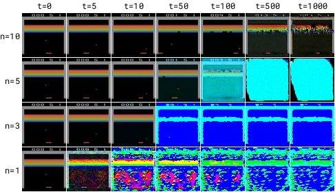
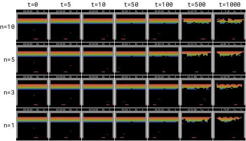
EDM vs DDPM 关键对比:n=3 步去噪时 DDPM 崩溃(=蓝屏),EDM 仍稳定(arXiv:2405.12399 Figure 3)
左: DDPM — n=3 时 t>10 就崩溃(蓝屏);右: EDM — n=3 时 t=1000 仍稳定
三个系列的工程权衡对比
| 维度 | Genie 1 | GAIA-2 | DIAMOND |
|---|---|---|---|
| 核心架构 | VQ-VAE + MaskGIT | Latent Diffusion DiT | U-Net 2D EDM |
| 参数量 | 10.7B total | 8.4B | 4.4M (Atari) / 381M (CSGO) |
| 动作学习 | 无监督 LAM | 结构化条件输入 | 直接嵌入 |
| 采样步数 | MaskGIT 8-16 iter | Flow Matching 50 | EDM 3 |
| 训练数据 | 680 万片段游戏 | 2500万 2秒驾驶片段 | 87 小时 CS:GO |
| 训练硬件 | 256 TPU v5p | 未公开 (H100 集群) | 单 RTX 4090 × 12 天 |
| 启示 | 无监督动作学习开创 | 双峰时间采样 + 多视角 | 预条件化让小模型逼近大模型 |
| 系统 | 参数 | 帧率 | 分辨率 | 特色 |
|---|---|---|---|---|
| GameNGen | ~860M | 20FPS | 320×240 | DOOM专用 |
| DIAMOND | 4.4-381M | ~10FPS | 原生 | 单RTX3090 |
| Oasis | 500M | 20FPS | ~360p | Diffusion Forcing |
| Genie 3 | 未公开 | 24FPS | 720p | 实时通用 |
关键数学公式
Genie LAM VQ 量化(STE 直通估计器)
最近邻分配:\(a_t = \arg\min_{i\in\{1,\dots,K\}}\,\|\tilde a_t - e_i\|_2^2\)
直通梯度:\(z_q = z_e + \operatorname{sg}(e_{a_t} - z_e)\)
VQ 损失:
\(\mathcal{L}_{\text{VQ}} = \|x - D(z_q)\|_2^2 + \underbrace{\|\operatorname{sg}(z_e) - e\|_2^2}_{\text{codebook}} + \beta\underbrace{\|z_e - \operatorname{sg}(e)\|_2^2}_{\text{commit}}\)
\(\beta=0.25\),codebook size \(K=8\) 迫使 LAM 学出 8 种最重要的动作模式。
MaskGIT 余弦掩码调度
迭代 n 步,第 s 步保留 ratio:
\(\operatorname{mask-ratio}(s) = \cos\!\left(\frac{\pi}{2}\cdot\frac{s}{N}\right)\)
对置信度最高的 top-k 个 token 在该步解除 mask。
GAIA-2 双峰 Logit-Normal 时间采样
训练 Flow Matching 时的 \(\tau\) 采样:
\(\tau = \sigma(z),\quad z\sim\begin{cases}\mathcal{N}(0.5,\,1.4^2) & \text{概率}\ 0.8\\ \mathcal{N}(-3.0,\,1.0^2) & \text{概率}\ 0.2\end{cases}\)
主峰覆盖中段去噪(模型主要降噪能力),次峰覆盖纯噪声附近(从零生成结构)。
Symlog 变换(自车动态)
速度、曲率等有符号量先经 symlog 压缩:
\(\operatorname{symlog}(v) = \operatorname{sign}(v)\cdot\ln(|v|+1)\)
例:\(v \in [-30, +30]\) m/s → \(\operatorname{symlog} \in [-3.43, +3.43]\);曲率类似。
AdaLN 动态量注入
\([\gamma,\beta] = \operatorname{MLP}\!\left(\left[\operatorname{symlog}(v_{\text{ego}}),\ \operatorname{symlog}(\kappa_{\text{ego}}),\ \tau_{\text{emb}}\right]\right)\)
\(\operatorname{AdaLN}(x) = \gamma\cdot\operatorname{LN}(x) + \beta\)
相机几何位置编码
每个 patch token 加上其所属相机的几何嵌入:
\(p_{\text{patch}} = \operatorname{PE}_{\text{spatial}}(r,c) + W\cdot\left[K_{\text{norm}};\ q_R;\ T;\ d_{\text{distort}}\right]\)
其中 K 是归一化内参(4 维)、q_R 是旋转四元数(4 维)、T 是平移(3 维)、distortion(5 维)。
DIAMOND EDM n=3 步 Heun 采样
\(\sigma\) schedule:
\(\sigma \in \{\sigma_0=80,\ \sigma_1=1.0,\ \sigma_2=0.002\}\)
每步应用 Heun 二阶修正:
\(d_i = \frac{x_i - D_\theta(x_i;\sigma_i,a,h)}{\sigma_i}\)
\(\tilde x_{i+1} = x_i + (\sigma_{i+1}-\sigma_i)\,d_i\)
\(x_{i+1} = x_i + (\sigma_{i+1}-\sigma_i)\cdot\tfrac{1}{2}\left(d_i + \tilde d_{i+1}\right)\)
n=3 关键:EDM 预条件化 + Heun 二阶修正 + 相邻帧高度相关(预测残差而非从噪声生成)。
DIAMOND Adaptive Group Norm(动作注入)
动作映射:\([s,b] = \operatorname{MLP}_a(a)\)
AGN 输出:\(\operatorname{AGN}(x,a) = (1+s)\cdot\operatorname{GN}(x) + b\)
Code 引用索引与可信度
✓=官方代码直接移植, △=基于论文描述重构, ⚠=推测填充 ——
注: 所有 "✓" 级代码的完整版本请参考对应 GitHub repo;本文的 PyTorch 伪代码经过简化以突出核心逻辑。
↑ 上级 · 02 技术架构与核心方法