---

Lecturer : Prof. Marco Hutter, Prof. Roland Siegwart, Dr Jesus Tordesillas

---

cheat sheet

online note

Kinematics

Position

• Cartesian coordinate : \(\boldsymbol \chi_{Pc}=\begin{bmatrix}x\\y\\z\end{bmatrix}, \bf r=\begin{bmatrix}x\\y\\z\end{bmatrix}\)
• Cylindrical coordinate : \(\boldsymbol \chi_{Pz}=\begin{bmatrix}\rho\\\theta\\z\end{bmatrix},_{\mathcal A}\bf r=\begin{bmatrix}\rho \cos \theta \\\rho \sin\theta\\z\end{bmatrix}\)
• Spherical coordinate : \(\boldsymbol \chi_{Ps}=\begin{bmatrix}r\\\theta\\\phi\end{bmatrix},_{\mathcal A}\bf r=\begin{bmatrix}r\cos\theta\sin\theta\\ r\sin\theta\sin\phi\\ r\cos\phi\end{bmatrix}\)

Linear Velocity

\[ \begin{aligned} \dot {\bf r} &= \textbf E_P(\boldsymbol \chi_P)\dot {\boldsymbol \chi}_P \\ \dot{\boldsymbol \chi}_P &= \textbf E_P^{-1}(\boldsymbol \chi_P)\dot {\textbf r} \end{aligned} \]

• Cartesian coordinate : \(\textbf E_{Pc} =\textbf E_{Pc}^{-1}= \mathbb I\)
• Cylindrical coordinate : \(\textbf E_{Pz}=\begin{bmatrix}\cos\theta&-\rho\sin\theta&0\\\sin\theta&\rho\cos\theta &0\\0&0&1\end{bmatrix}\), \(\textbf E_{Pz}^{-1} = \begin{bmatrix}\cos\theta&\sin\theta&0\\-\sin\theta/\rho&\cos\theta/\rho &0\\0&0&1\end{bmatrix}\)
• Spherical Coordinate : \(\textbf E_{Ps}=\begin{bmatrix}\cos\theta\sin\phi & -r\sin\phi\sin\theta & r\cos\phi\cos\theta\\\sin\phi\sin\theta & r\cos\theta\sin\phi & r\cos\phi \sin\theta\\ \cos\phi & 0 & -r\sin\phi\end{bmatrix}\), \(\textbf E_{Ps}^{-1}=\begin{bmatrix}\cos\theta\sin\phi & \sin\phi\sin\theta&\cos\phi\\-\sin\theta/(r\sin\phi)&\cos\theta/(r\sin\phi)&0\\(\cos\phi\cos\theta)/r&(\cos\phi\sin\theta)/r& -\sin\phi /r\end{bmatrix}\)

Rotation

• Passive Rotation : \(_{\mathcal A}\textbf u = \textbf C_{\mathcal{AB}}\cdot_{\mathcal B}\textbf u\) ; Active Rotation : \(_{\mathcal A}\textbf v=\textbf R\cdot _{\mathcal A}\textbf u\)

• Elementary Rotation : \(\textbf C_x(\varphi)=\begin{pmatrix}1&0&0\\0&\cos\varphi&-\sin\varphi\\0&\sin\varphi&\cos\varphi\end{pmatrix}\) , \(\textbf C_y(\varphi) = \begin{pmatrix}\cos\varphi & 0 &\sin\varphi \\0&1&0\\-\sin\varphi&0&\cos\varphi\end{pmatrix}\) , \(\textbf C_z(\varphi)=\begin{pmatrix}\cos\varphi&-\sin\varphi&0\\\sin\varphi&\cos\varphi&0\\0&0&1\end{pmatrix}\)

• Euler Angle

• ZYZ Euler Angle (yaw-pitch-yaw) : \(\textbf C = \textbf C_{z_1}\textbf C_{y}\textbf C_{z_2}\) , \(\boldsymbol \chi_{R,eulerZYZ}=\begin{pmatrix}\text{atan}(c_{23}/c_{13})\\ \text{atan}(\sqrt{c_{13}^2+c_{23}^2}/c_{33})\\\text{atan}(c_{32}/(-c_{31}))\end{pmatrix}\)
• ZXZ Euler Angle (yaw-roll-yaw) : \(\textbf C = \textbf C_{z_1}\textbf C_{x}\textbf C_{z_2}\) , \(\boldsymbol \chi_{R,eulerZXZ}=\begin{pmatrix}\text{atan}(c_{13}/(-c_{23}))\\ \text{atan}(\sqrt{c_{13}^2+c_{23}^2}/c_{33})\\\text{atan}(c_{31}/c_{32})\end{pmatrix}\)
• ZYX Euler Angle (yaw-pitch-roll) : \(\textbf C = \textbf C_{z}\textbf C_{y}\textbf C_{x}\) , \(\boldsymbol \chi_{R,eulerZYX}=\begin{pmatrix}\text{atan}(c_{21}/c_{11})\\ \text{atan}(-c_{31}/\sqrt{c_{32}^2+c_{33}^2})\\\text{atan}(c_{32}/c_{33})\end{pmatrix}\)
• XYZ Euler Angle (roll-pitch-yaw) : \(\textbf C = \textbf C_{x}\textbf C_{y}\textbf C_{z}\) , \(\boldsymbol \chi_{R,eulerXYZ}=\begin{pmatrix}\text{atan}(-c_{23}/c_{33})\\ \text{atan}(c_{13}/\sqrt{c_{11}^2+c_{12}^2})\\\text{atan}(-c_{12}/c_{11})\end{pmatrix}\)
• Angle Axis : \(\boldsymbol \chi_{R,AngleAxis}=\begin{pmatrix}\theta\\\textbf n\end{pmatrix},\Vert \textbf n\Vert=1\)
• Euler Vector/ Rotation Vector : \(\varphi = \theta\cdot \textbf n\in \mathbb R^3\)
• \(\textbf C_{\mathcal {AB}} = \begin{bmatrix}n_x^2(1-c_\theta)+c_\theta&n_xn_y(1-c_\theta)-n_zs_\theta&n_xn_z(1-c_\theta)+n_ys_\theta\\n_xn_y(1-c_\theta)+n_zs_\theta& n_y^2(1-c_\theta)+c_\theta & n_yn_z(1-c_\theta)-n_xs_\theta\\ n_xn_z(1-c_\theta)-n_ys_\theta&n_yn_z(1-c_\theta)+n_xs_\theta&n_z^2(1-c_\theta)+c_\theta\end{bmatrix}\)
• \(\theta=\cos^{-1}\left(\frac{\text{Tr}(\textbf C)-1}{2}\right)\) , \(\textbf n=\frac{1}{2\sin\theta}\begin{pmatrix}c_{32} - c_{23}\\c_{13}-c_{31}\\c_{21}-c_{12}\end{pmatrix}\)
• Unit Quaternions : \(\boldsymbol \chi_{R,quat}=\boldsymbol \xi=\begin{pmatrix}\xi_0\\\check {\boldsymbol \xi}\end{pmatrix}, \sum_{i=0}^3\xi_i^2=1\)
• \(\xi_0 = \cos\left(\frac{\Vert \varphi\Vert}{2}\right)=\cos\left(\frac{\theta}{2}\right)\) , \(\check{\boldsymbol \xi}=\sin\left(\frac{\Vert\varphi\Vert}{2}\right)\frac{\varphi}{\Vert\varphi\Vert} = \sin\left(\frac{\theta}{2}\right)\textbf n\)
• \(\textbf C_{\mathcal {AD}} = \mathbb I + 2\xi_0\left[\check{\boldsymbol \xi}\right]_\times + 2\left[\check{\boldsymbol\xi}\right]^2_{\times} = (2\xi_0^2-1)\mathbb I+2\xi_0\left[\check{\boldsymbol \xi}\right]_\times + 2\check {\boldsymbol \xi}\check{\boldsymbol \xi}^\top\) where \(\left[\check {\boldsymbol \xi}\right]_\times = \begin{bmatrix}0&-\xi_3&\xi_2\\\xi_3&0&-\xi_1\\-\xi_2&\xi_1&0\end{bmatrix}\)
• \(\boldsymbol \xi = \frac{1}{2}\begin{pmatrix}\sqrt{\text{Tr}(\textbf C)+1}\\\text{sgn}(c_{32}-c_{23})\sqrt{c_{11}-c_{22}-c_{33}+1}\\\text{sgn}(c_{13}-c_{31})\sqrt{c_{22}-c_{33}-c_{11}+1}\\\text{sgn}(c_{21}-c_{12})\sqrt{c_{33}-c_{11}-c_{22}+1}\end{pmatrix}\)
• Inverse : \(\boldsymbol \xi^{-1} = \boldsymbol \xi^\top=\begin{pmatrix}\xi_0\\-\check{\boldsymbol \xi}\end{pmatrix}\)
• Multiplication : \(\boldsymbol \xi_{\mathcal{AC}} = \underbrace{\begin{bmatrix}\xi_0 & -\check{\boldsymbol \xi}^\top\\ \check{\boldsymbol \xi}&\xi_0\mathbb I+\left[\check {\boldsymbol \xi}\right]_\times\end{bmatrix}}_{\textbf M_l(\boldsymbol \xi_{\mathcal AB})}\boldsymbol \xi_{\mathcal {BC}} = \underbrace{\begin{bmatrix}\xi_0 & -\check{\boldsymbol \xi}^\top\\\check{\boldsymbol \xi}&\xi_0\mathbb I-\left[\check {\boldsymbol \xi}\right]_\times\end{bmatrix}}_{\textbf M_r(\boldsymbol \xi _{\mathcal BC})}\boldsymbol \xi_{\mathcal {AB}}\)
• Vector Rotation : \(\begin{pmatrix}0\\_{\mathcal A}\textbf r\end{pmatrix} = \textbf M_l(\boldsymbol \xi_{\mathcal {AB}})\textbf M_r(\xi_{\mathcal {AB}}^\top)\begin{pmatrix}0\\_{\mathcal B }\textbf r\end{pmatrix}\)
• Degree of Freedom : 3

Angular Velocity

\[ _{\mathcal A}\omega_{\mathcal{AB}} = \textbf E_R(\boldsymbol \chi_R)\cdot \dot {\boldsymbol \chi}_R \]

• Transform : \(\left[_{\mathcal B}\omega_{\mathcal {AB}}\right]_\times = \textbf C_{\mathcal {BA}}\cdot \left[_{\mathcal A}\omega_{\mathcal {AB}}\right]_\times\cdot \textbf C_{\mathcal {AB}}\)
• Euler Angle: \(\textbf E_{R,euler \alpha\beta\gamma} = \begin{bmatrix}_{\mathcal A}\textbf e_A^{\mathcal \alpha}& _{\mathcal A}\textbf e_\beta^{\mathcal A'}& _{\mathcal A}\textbf e_\gamma^{\mathcal A''}\end{bmatrix}\)
• ZYZ : \(\textbf E_{R,eulerZYZ} = \begin{bmatrix}0&-\sin z_1&\cos z_1\sin y\\0 & \cos z_1 & \sin z_1\sin y\\ 1 & 0 & 0\end{bmatrix}\) , \(\textbf E^{-1}_{R,eulerZYZ} = \begin{bmatrix}-\cos y\cos z_1/\sin y & -\cos y \sin z_1/\sin y & 1\\ -\sin z_1 & \cos z_1 & 0\\ \cos z_1/\sin y & \sin z_1/ \sin y & 0\end{bmatrix}\)
• ZXZ : \(\textbf E_{R,euler ZXZ}=\begin{bmatrix}0&\cos z_1&\sin z_1 \sin x\\ 0 & \sin z_1 & -\cos z_1 \sin x\\ 1 & 0 & \cos x\end{bmatrix}\) , \(\textbf E^{-1}_{R,eulerZXZ} = \begin{bmatrix}-\cos x\sin z_1/\sin x & \cos x\cos z_1/\sin x & 1\\ \cos z_1 & \sin z_1 & 0 \\ \sin z_1 /\sin x & -\cos z_1/ \sin x & 0\end{bmatrix}\)
• ZYX : \(\textbf E_{R,eulerZYX} = \begin{bmatrix}0 & -\sin z & \cos y \cos z \\ 0 & \cos z & \cos y \sin z\\ 1 & 0 & -\sin y\end{bmatrix}\) , \(\textbf E^{-1}_{R,eulerZYX} = \begin{bmatrix}\cos z \sin y /\cos y & \sin y \sin z /\cos y & 1\\ -\sin z & \cos z & 0 \\ \cos z / \cos y & \sin z /\cos y & 0\end{bmatrix}\)
• XYZ : \(\textbf E_{R,eulerXYZ}=\begin{bmatrix}1 & 0 & \sin y \\ 0 & \cos x & -\cos y \sin x\\ 0 & \sin x & \cos x \cos y \end{bmatrix}\), \(\textbf E^{-1}_{R,euler XYZ}=\begin{bmatrix}1&\sin x\sin y/\cos y & -\cos x\sin y /\cos y\\ 0 & \cos x & \sin x\\ 0 & -\sin x /\cos y & \cos x /\cos y\end{bmatrix}\)
• Angular Axis : \(\textbf E_{R,angleaxis}=\begin{bmatrix}\textbf n& \sin\theta\mathbb I+(1-\cos\theta)\left[\textbf n\right]_\times\end{bmatrix}\) , \(\textbf E_{R,angleaxis}^{-1}=\begin{bmatrix}\textbf n^\top\\ -\frac{1}{2}\frac{\sin\theta}{1-\cos\theta}\left[\textbf n\right]^2_\times-\frac{1}{2}\left[\boldsymbol n \right]_\times\end{bmatrix}\)
• Rotation Vector : \(\textbf E_{R,rotationvector}=\begin{bmatrix}\mathbb I+\left[\varphi\right]_\times\left(\frac{1-\cos\Vert\varphi\Vert}{\Vert\varphi\Vert^2}\right)+\left[\varphi\right]_\times^2\left(\frac{\Vert \varphi \Vert -\sin\Vert \varphi\Vert}{\Vert \varphi\Vert^3}\right)\end{bmatrix}\) , \(\textbf E_{R,rotationvector}^{-1}=\left[\mathbb I -\frac{1}{2}\left[\varphi\right]_\times + \left[\varphi\right]^2_\times\frac{1}{\Vert\varphi\Vert^2}\left(1-\frac{\Vert\varphi\Vert}{2}\frac{\sin\Vert\varphi\Vert}{1-\cos\Vert\varphi\Vert}\right)\right]\)
• Unit Quaternions : \(\textbf E_{R,quat}=2\textbf H(\boldsymbol \xi)\) , \(\textbf E_{R,quat}^{-1}=\frac{1}{2}\textbf H(\boldsymbol \xi)^\top\), with \(\textbf H(\boldsymbol \xi) = \begin{bmatrix}-\check{\boldsymbol \xi}&\left[\check{\boldsymbol \xi}\right]_\times + \xi_0 \mathbb I\end{bmatrix}\in \mathbb R^{3\times 4}\)

Transformation

\(\textbf T_{\mathcal {AB}} = \begin{bmatrix}\textbf C_{\mathcal {AB}} & _{\mathcal A}\textbf r_{\mathcal{AB}}\\\textbf 0 & 1\end{bmatrix}\)

• Inverse \(\textbf T_{\mathcal {AB}}^\top = \begin{bmatrix}\textbf C^\top_{\mathcal{AB}} &\overbrace{-\textbf C_{\mathcal {AB}}^\top \textbf r_{\mathcal {AB}}}^{_{\mathcal B}\textbf r_{\mathcal {BA}}}\\ \textbf 0 & 1\end{bmatrix}\)
• Multiplication : \(\textbf T_{\mathcal {AC}}=\textbf T_{\mathcal {AB}} \textbf T_{\mathcal {BC}}\)

Transformation Acceleration

• Acceleration : \(\ddot {\textbf r}_{P} = \ddot{\textbf r}_{B} + \dot \omega_B\times \textbf r_{BP } + \omega_B\times(\omega_B\times \textbf r_{BP})\)
• Moving System \(\mathcal B\) : \(_{\mathcal B}\dot{\textbf r}_{\mathcal {BP}} = _{\mathcal B}\dot{\textbf r_{\mathcal{AP}}} + _{\mathcal B}\omega_{\mathcal {AB}}\times _{\mathcal B}\textbf r_{\mathcal {AP}}\)

Task-space Coordinate

• End-Effector/Operational Space Coordinate : \(\boldsymbol \chi_e=\begin{pmatrix} \boldsymbol \chi_{e_P}\\ \boldsymbol \chi_{e_R}\end{pmatrix}\)

forward Kinematics

\[ \textbf T_{\mathcal {IE}}(\textbf q) = \textbf T_{\mathcal{I}0}\cdot\prod_{k=1}^{n_j}\textbf T_{k-1,k}(q_k)\cdot \textbf T_{n_j\mathcal E} \]

Differential Kinematics

$\(\dot{\boldsymbol \chi}_e = \textbf J_{eA}(\textbf q)\dot {\textbf q}\)$

$\(\ddot{\boldsymbol\chi}_e = \textbf J_{eA}(\textbf q)\ddot {\textbf q} + \dot{\textbf J}_{eA}(\textbf q)\dot{\textbf q}\)$

Analytical Jacobian

\[\textbf J_{eA}=\begin{bmatrix}\textbf J_{eA_P}\\\textbf J_{eA_R}\end{bmatrix}=\begin{bmatrix}\frac{\partial \boldsymbol \chi_{e_P}}{\partial \textbf q}\\ \frac{\partial \boldsymbol \chi _{e_R}}{\partial \textbf q}\end{bmatrix}\in \mathbb R^{m_e\times n_j}\]

• \(\dot{\boldsymbol \chi}_e = \textbf J_{eA}(\textbf q)\dot {\textbf q}\)

Geometric Jacobian

\[\textbf J_{e0}\in \mathbb R^{6\times n_j}\]

• \(\textbf w_e = \textbf J_{e0}(\textbf q) \boldsymbol \omega\)
• Addition : \(\textbf J_{c0} = \textbf {J}_{b0} +\textbf J_{bc0}\)
• from Analytical Jacobian : \(\textbf J_{e0}(\textbf q)=\textbf E_e(\boldsymbol\chi)\textbf J_{eA}(\textbf q)\), where \(\textbf E_e(\boldsymbol\chi)=\begin{bmatrix}\textbf E_P&\\&\textbf E_R\end{bmatrix}\in \mathbb R^{6\times m_e}\)

Revolute Joint

\[_{\mathcal I}\textbf J_{e0}=\begin{bmatrix}_{\mathcal I}\textbf n_1\times _{\mathcal I}\textbf r_{1(n+1)}&\cdots & _{\mathcal I}\textbf n_n\times _{\mathcal I}\textbf r_{n(n+1)}\\_{\mathcal I}\textbf n_1&\cdots & _{\mathcal I}\textbf n_n\end{bmatrix}\]

Prismatic Joint

\[_{\mathcal I}\textbf J_{e0}=\begin{bmatrix}_{\mathcal I}\textbf n_1&\cdots & _{\mathcal I}\textbf n_n\\ \textbf 0 &\cdots &\textbf 0\end{bmatrix}\]

Inverse Differential Kinematics

$\(\dot {\textbf q} = \textbf J_{e0}^+\textbf w_e^*\)$

where \(\textbf w_e^*\) is (desired) end-effector velocity

• full column rank $m\ge n $ : \(A^+ = (A^\top A)^{-1}A^\top=\underset{A}{\text{argmin}}\Vert Ax-b\Vert_2^2\)
• full row rank \(m\le n\) : \(A^+ = A^\top (AA^\top)^{-1}\)
• damped : \(A^+_d = A^\top (AA^\top + \lambda ^2 \mathbb I)^{-1}=\underset{A}{\text{argmin}}\Vert Ax-b\Vert_2^2+\lambda^2 \Vert x\Vert_2^2\)
• singularity : \(\text{rank}(\textbf J_{e0})<6\)
• solution : 1. damped, 2. redundancy

Multi-task Inverse Differential Kinematics

\[task_i =\{\textbf J_i, \textbf w_i^*\}\]

Equal Priority

\[\dot {\textbf q} =\underbrace{\begin{bmatrix}\textbf J_1\\\vdots\\\textbf J_{n_t}\end{bmatrix}^+}_{\bar{\textbf J}^+ }\underbrace{\begin{pmatrix}\textbf w_1^*\\\vdots\\ \textbf w^*_{n_t}\end{pmatrix}}_{\bar{\textbf w}} = \underset{\dot q}{\text{argmin}}\Vert \bar{\textbf J}\dot{\textbf q}-\bar{ \textbf w}\Vert_2\]

• task weighted : \(\bar{\textbf J}^{+W} = (\bar{\textbf J}^\top \textbf W\bar{\textbf J})^{-1}\bar{\textbf J}^\top \textbf W\) where \(\textbf W=\text{diag}(w_1,\cdots,w_m)\)

Prioritization

\[\dot {\textbf q} = \sum_{i=1}^{m}\bar{\textbf N}_{i-1}\dot {\textbf q}_i\]

where \(\dot {\textbf q}_i = (\textbf J_i\bar{\textbf N}_{i-1})^+\left(\textbf w_i^* - \textbf J_i\sum_{k=1}^{i-1}\bar{\textbf N}_{k-1}\dot {\textbf q}_k\right)\) where \(\bar{\textbf N}_i=\mathbb I - \textbf J_i^+\textbf J_i\) is the null space

• example \(m=2\) : \(\dot {\textbf q}=\textbf J_1^+\textbf w_1^* + \textbf N_1(\textbf J_2\textbf N_1)^+(\textbf w_2^* - \textbf J_2\textbf J_1^+\textbf w_1^*)\)

Inverse Kinematics

Numerical Solution

1. \(\textbf q\gets \textbf q^0\)
2. while \(\Vert \boldsymbol \chi _e^* - \boldsymbol \chi _e(\textbf q)\Vert> \epsilon\) do
   1. \(\Delta \boldsymbol \chi_e\gets \boldsymbol \chi_e^*-\boldsymbol \chi_e(\textbf q)\) where \(_{\mathcal I} \Delta \varphi = \text{rotVec}(\textbf C_{\mathcal{IB}}\textbf C_{\mathcal {IA}}^\top)\)
   2. \(\textbf q\gets \textbf q + \alpha \textbf J_{eA}^+(\textbf q)\Delta \boldsymbol \chi_e\)

Trajectory Control

• Position : \(\dot q^* = \textbf J^+_{e0_P}(\textbf q^t)\cdot (\dot{\textbf r}_e^*(t) + k_{p_P}\Delta \textbf r_e^t)\)
• Orientation : \(\dot {\textbf q}^* = \textbf J_{e0_R}^+(\textbf q^t)\cdot (\omega_e^*(t)+k_{p_R}\Delta \varphi)\)

Floating Base kKinematics

\(n_n=n_b+n_j\), \(n_b\) un-actuated base coordinate + \(n_j\) actuated joint coordinate

Generalized Velocity

\[\textbf u = \begin{pmatrix}_{\mathcal I}\textbf v_{ \mathcal B}\\_{\mathcal B}\boldsymbol \omega_{\mathcal {IB}}\\\dot \varphi_1\\\vdots \\ \dot\varphi_{n_j}\end{pmatrix} \in \mathbb R^{6+n_j}\]

where \(\mathcal B\) is the floating base, \(\mathcal I\) is the inertial frame

Forward Kinematics

\[_{\mathcal I}\textbf r_{\mathcal{IQ}}(\textbf q) = _{\mathcal I}\textbf r_{\mathcal {IB}}(\textbf q) + \textbf C_{\mathcal{IB}}(\textbf q)\cdot_{\mathcal B}\textbf r_{\mathcal{BQ}}(\textbf q)\]

where \(\textbf C_{\mathcal{IB}}\) describe the orientation of the floating base \(\mathcal B\)

Differential Kinematics

\[_{\mathcal I}\textbf J_Q(\textbf q) = \begin{bmatrix}_{\mathcal I}\textbf J_P \\ _{\mathcal I}\textbf J_R\end{bmatrix}= \begin{bmatrix}\mathbb I & -\textbf C_{\mathcal {IB}}\cdot\left[_{\mathcal B}\textbf r_{BQ}\right]_\times & \textbf C_{\mathcal{IB}}\cdot _{\mathcal B}\textbf J_{P_{q_j}}(\textbf q_j)\\\textbf 0 & \textbf C_{\mathcal {IB}}& \textbf C_{\mathcal{IB}}\cdot _{\mathcal B}\textbf J_{R_{q_j}}(\textbf q_j)\end{bmatrix}\]

Contact and Constraint

\[\textbf r_c = \text{const}\quad\dot{\textbf r}=\ddot{\textbf r}_c=0\]

\[\Leftrightarrow\]

\[_{\mathcal I}\textbf J_{C_i}\textbf u=\textbf 0 $$ $$ _{\mathcal I}\textbf J_{C_i}\dot {\textbf u}+_{\mathcal I}\dot{\textbf J}_{C_i}\textbf u = \textbf 0\]

where \(\textbf J_c\in \mathbb R^{3n_c\times n_n}\) , \(n_c\) is the number of contacts

Dynamics

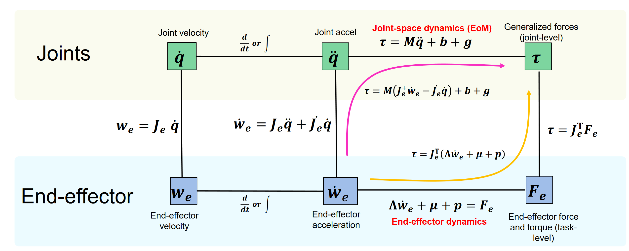
Generalized Equation of Motion

\[ \textbf M(\textbf q)\ddot{\textbf q} + \textbf b(\textbf q,\dot{\textbf q})+\textbf g(\textbf q) = \textbf S^\top\tau + \textbf J_c(\textbf q)^\top \textbf F_c \]

• \(\textbf q,\dot{\textbf q},\ddot{\textbf q}\in \mathbb R^{n_q}\) : generalized position, velocity, acceleration
• \(\textbf M(\textbf q)\in \mathbb R^{n_q\times n_q}\) : \(\textbf M=\sum_{i=1}^{n_b}(_{\mathcal A}\textbf J_{S_i}^\top m_{\mathcal A}\textbf J_{S_i}+_{\mathcal B}\textbf J_{R_i}^\top~ _{\mathcal B}\Theta_{S_i} ~_{\mathcal B}\textbf J_{R_i})\) generalized mass matrix
• \(\textbf b(\textbf q,\dot{\textbf q})\in \mathbb R^{n_q}\) : \(\textbf b=\sum_{i=1}^{n_b}\left(_{\mathcal A}\textbf J_{S_i}^\top m_{\mathcal A}\dot{\textbf J}_{S_i}\dot{\textbf q}+~_{\mathcal B}\textbf J_{R_i}^\top\left(_{\mathcal B}\Theta_{\mathcal B}\dot{\textbf J}_{R_i}\dot{\textbf q}+~_{\mathcal B}\boldsymbol\Omega_{S_i}\times ~_{\mathcal B}\Theta_{S_i}~_{\mathcal B}\boldsymbol \Omega_{S_i}\right)\right)\) coriolis and centrifugal terms, where \(\boldsymbol \Omega_{S_i} = \textbf J_{R_i}\dot{\textbf q}\)
• \(\textbf g(\textbf q)\in \mathbb R^{n_q}\) : \(\textbf g=\sum_{i=1}^{n_b}-~_{\mathcal A}\textbf J_{S_i}^\top ~_{\mathcal A}\textbf F_{g,i}\) gravitational terms

• Example : \(\textbf g = \sum_i -\textbf J_i^\top m_i\begin{pmatrix}0\\0\\-9.81\end{pmatrix}\)

• \(\tau\in \mathbb R^{n_\tau}\) : generalized torques acting in direction of generalized coordinate \(\tau = \sum_{k=1}^{n_A} \tau_{a,k}\tau_{ext}\) external generalized forces,

• actuator generalized force \(\tau_{a,k}=(\textbf J_{S_k} - \textbf J_{S_{k-1}})^\top\textbf F_{a,k}+(\textbf J_{R_k}-\textbf J_{R_{k-1}})^\top \textbf T_{a,k}\), \(\textbf T\) is torque here
• external generalized force \(\tau_{ext}=\sum_{j=1}^{n_{f,ext}}\textbf J_{P,j}^\top \textbf F_j+\sum_{j=1}^{n_{m,ext}}\textbf J_{R,j}^\top\textbf T_{ext, j}\)
• \(\textbf S\in \mathbb R^{n_\tau\times n_q}\) : selection matrix of actuated joints
• \(\textbf F_c\in \mathbb R^{n_c}\) : external Cartesian forces (e.g. from contacts)
• Soft Contact Model : \(\textbf F_c = k_p(\textbf r_c-\textbf r_{c0})+k_d\dot{\textbf r}_c\)
• Contact Force from Constraint \(\textbf r_c = \text{const}\quad\dot{\textbf r}=\ddot{\textbf r}_c=0\) : \(\textbf F_c = (\textbf J_c\textbf M^{-1}\textbf J_c^\top)^{-1}\left(\textbf J_c\textbf M^{-1}(\textbf S^{\top}\tau-\textbf b-\textbf g)+\dot{\textbf J}_c\textbf u\right)\)
• \(\textbf J_c(\textbf q)\in \mathbb R^{n_c\times n_q}\) : Geometric Jacobian corresponding to external force
• Kinect Energy : \(\mathcal T (\textbf q,\dot{\textbf q})=\frac{1}{2}\dot{\textbf q}^\top\underbrace{\left(\sum_{i=1}^{n_b}(\textbf J_{S_i}^\top m\textbf J_{S_i}+\textbf J_{R_i}^\top \Theta_{S_i}\textbf J_{R_i})\right)}_{\textbf M(\textbf q)}\dot {\textbf q}\)
• Potential Energy : \(\mathcal U_g = -\sum_{i=1}^{n_b} \textbf r_{S_i}^\top \textbf F_{g_i}\)

Dynamics of Floating Base System

Contact Force

• Soft Contact : \(\textbf F_c = k_p (\textbf r_c - \textbf r_{c0}) + k_d \dot{\textbf r}_c\)

• Constraint Contact : \(\textbf r_c = \text{const}\), \(\dot{\textbf r}_c =\textbf J_c\textbf u = \textbf 0\), \(\ddot{\textbf r}_c = \textbf J_c \dot{\textbf u}+\dot{\textbf J}_c\textbf u = \textbf 0\)

\(\textbf F_c = (\textbf J_c\textbf M^{-1}\textbf J_c^\top)^{-1}\left(\textbf J_c\textbf M^{-1}(\textbf S^\top \tau -\textbf b-\textbf g) + \dot{\textbf J}_c \textbf u\right)\)

Constraint Consistent Dynamics :

• \(\textbf N_c = \mathbb I - \textbf M^{-1}\textbf J_c^\top (\textbf J_c \textbf M^{-1}\textbf J_c^\top)^{-1} \textbf J_c\)
• \(\textbf N_c^\top (\textbf M\dot{\textbf u}+\textbf b+\textbf g) = \textbf N_c^\top \textbf S^\top \tau\)

Impulse Transfer

• end-effector inertia : \(\boldsymbol \Lambda_c = (\textbf J_c\textbf M^{-1}\textbf J_c^\top)^{-1}\)
• instantaneous change : \(\Delta u =\textbf u^+-\textbf u^0= - \textbf M^{-1}\textbf J_c^\top (\textbf J_c\textbf M^{-1}\textbf J_c^\top)^{-1}\textbf J_c\textbf u^{-}\)
• post-impact generalized velocity : \(\textbf u^+ = \textbf N_c \textbf u^{-1}\)
• Energy Loss : \(E_{loss} = -\frac{1}{2}\Delta \textbf u^\top_c\boldsymbol \Lambda_c \Delta \textbf u\)

Joint Space Dynamic Control

Gravity Compensation

\[\tau^* = k_p(\textbf q^* - \textbf q) + k_d(\dot{\textbf q}^*-\dot{\textbf q})+\textbf g(\textbf q)\]

Inverse Dynamics Control

\[\ddot{\textbf q}^* = k_p(\textbf q^*-\textbf q)+k_d(\dot{\textbf q}^*-\dot{\textbf q})$$ $$\omega=\sqrt{k_p},D=\frac{k_d}{2\sqrt{k_p}}\]

Task Space Dynamic Control

$\(\dot {\textbf w}_e = \begin{pmatrix}\ddot{\textbf r}\\\dot{\boldsymbol \omega}\end{pmatrix}=\textbf J_e\ddot{\textbf q} + \dot{\textbf J}_e\dot{\textbf q}\)$

Multi-task Decomposition

• Equal Priority : \(\ddot {\textbf q} =\begin{bmatrix}\textbf J_1\\\vdots\\\textbf J_{n_t}\end{bmatrix}^+\left(\begin{pmatrix}\dot{\textbf w_1}^*\\\vdots\\ \dot{\textbf w^*_{n_t}}\end{pmatrix} - \begin{bmatrix}\dot{\textbf J}_1\\\vdots\\\dot{\textbf J}_{n_t}\end{bmatrix}\dot{\textbf q}\right)\)
• Prioritization : \(\ddot {\textbf q} = \sum_{i=1}^{n_t}\textbf N_{i}\ddot {\textbf q}_i\) where \(\ddot {\textbf q}_i = (\textbf J_i\textbf N_{i})^+\left(\dot{\textbf w_i}^* - \dot{\textbf J}_i\dot{\textbf q}-\textbf J_i\sum_{k=1}^{i-1}\textbf N_k\ddot {\textbf q}_k\right)\) where \(\textbf N_i=\mathbb I - \textbf J_i^+\textbf J_i\) is the null space

End-effector Dynamics

$\(\Lambda _e \dot{\textbf w}_e + \boldsymbol \mu + \textbf p=\textbf F_e\)$

• \(\Lambda_e = (\textbf J_e\textbf M^{-1}\textbf J_e^\top)^{-1}\) : end-effector inertia
• \(\boldsymbol \mu = \Lambda_e\textbf J_e\textbf M^{-1}\textbf b - \Lambda_e \dot{\textbf J}_e\dot{\textbf q}\) : end-effector centrifugal/Coriolis
• \(\textbf p = \Lambda_e \textbf J_e\textbf M^{-1}\textbf g\) : end-effector gravitational
• joint torque \(\tau = \textbf J_e^\top \textbf F_e\)

End-effector Motion Control

\[\tau^* = \textbf J^\top(\Lambda_e\dot{\textbf w}_e^*+\boldsymbol \mu + \textbf p)=\textbf J^\top \Lambda_e\dot{\textbf w}_e^*+\textbf b-\textbf J^\top \Lambda_e\dot{\textbf J}_e\dot{\textbf q}+\textbf g\]

Operational Space Control

\[\tau^*=\textbf J^\top(\Lambda \textbf S_M\dot{\textbf w}_e + \textbf S_F\textbf F_c + \boldsymbol \mu +\textbf p)\]

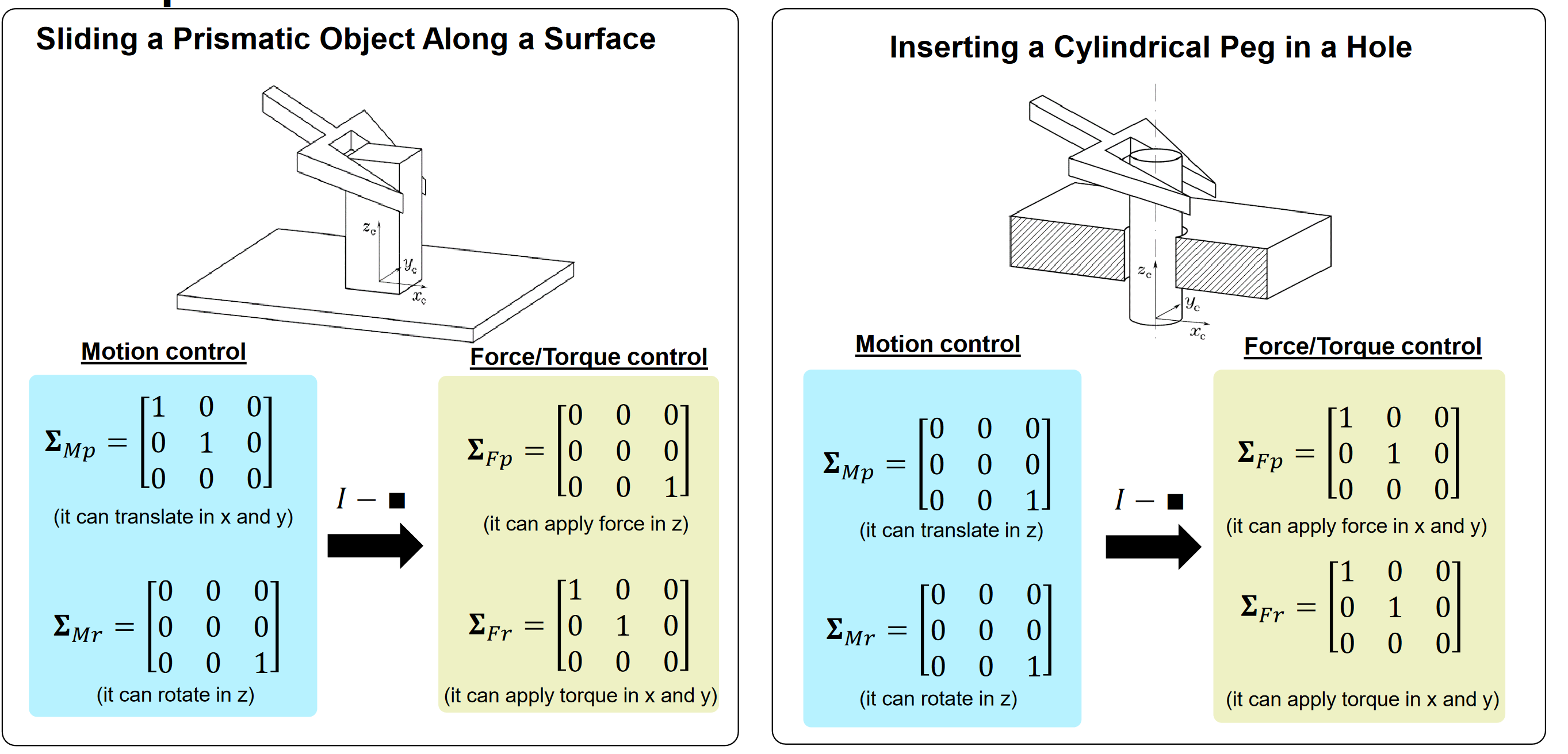
• \(\Sigma_p =\begin{bmatrix}\sigma_{px}&0&0\\0&\sigma_{py}&0\\0&0&\sigma_{pz}\end{bmatrix}\) , \(\Sigma_r = \begin{bmatrix}\sigma_{rx}&0&0\\0&\sigma_{ry}&0\\0&0&\sigma_{rz}\end{bmatrix}\) where \(\sigma_i=1\) if the axis is free of motion, otherwise \(0\)

• \(\textbf S_M=\begin{bmatrix}\textbf C^\top \Sigma_p\textbf C&0\\0&\textbf C^\top \Sigma_r \textbf C\end{bmatrix}\) , \(\textbf S_F=\begin{bmatrix}\textbf C^\top (\mathbb I -\Sigma_p)\textbf C&0 \\ 0& \textbf C^\top (\mathbb I-\Sigma_r)\textbf C\end{bmatrix}\)

  

Inverse Dynamics for Floating-Base Systems

Hierarchical Least Square Optimization

$\(\underset{\textbf x}{\text{min}}\Vert \textbf A_i\textbf x - \textbf b_i\Vert_2\)$

with priority normally \(\textbf x = \begin{bmatrix}\ddot {\textbf q}^\top &\boldsymbol\tau^\top & _{\mathcal I}\textbf F_E^\top\end{bmatrix}^\top\)

1. \(n_T\) : number of tasks
2. \(\textbf x=\textbf 0\) : initial optimal solution
3. \(\textbf N_1 = \mathbb I\) : initial null-space projector
4. for \(i=1\to n_T\) do
   1. \(\textbf x_i\gets (\textbf A_i\textbf N_i)^+(\textbf b_i-\textbf A_i\textbf x)\)
   2. \(\textbf x\gets \textbf x + \textbf N_i\textbf x_i\)
   3. \(\textbf N_{i+1}=\mathcal N\left(\left[\textbf A_1^\top\cdots\textbf A_i^\top\right]^\top\right)\) : null-space, normally \(\mathcal N(\textbf A)=\mathbb I-\textbf A^+ \textbf A\) , \(\mathcal N(\textbf A)\textbf A = \textbf 0\)

Legged Robot

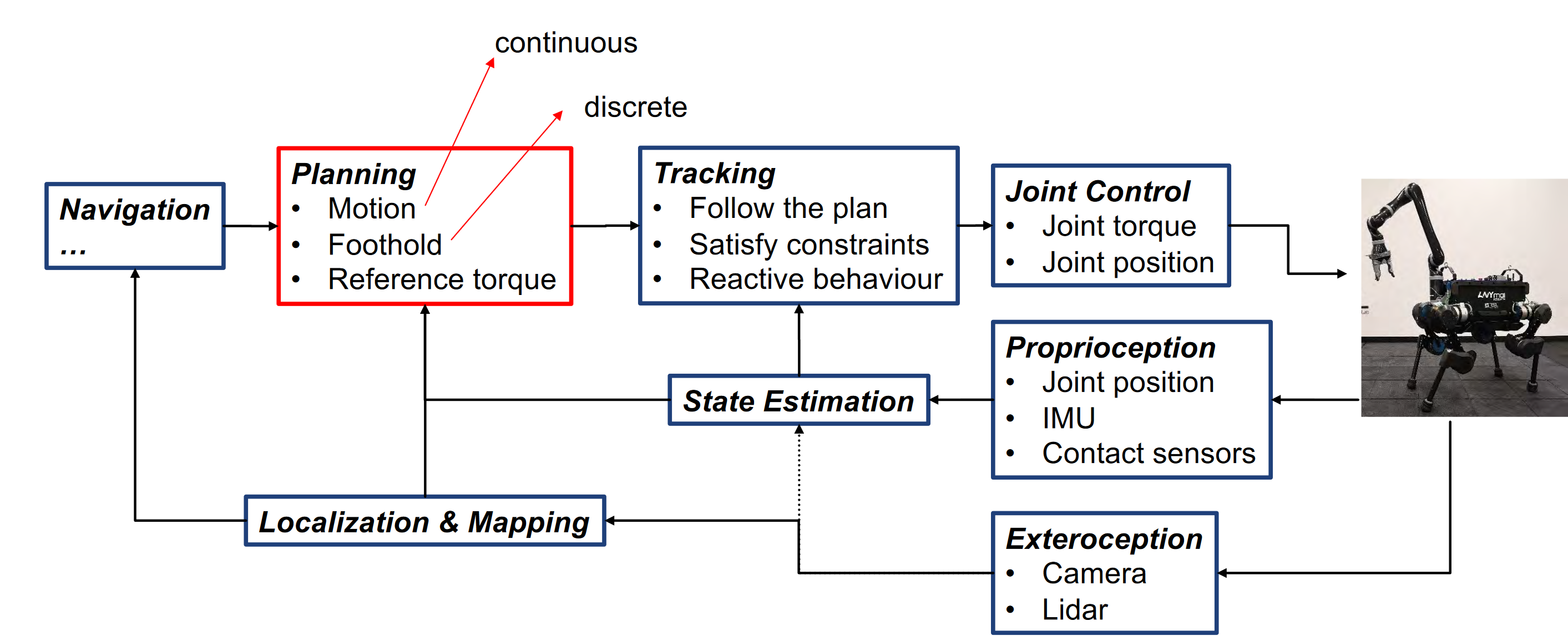
Input : \(\textbf q,\dot{\textbf q}\)

Optimization Target : \(\ddot {\textbf q}, \textbf F_c, \boldsymbol \tau\)

Tasks :

1. Equation of Motion : \(\begin{bmatrix}\textbf M(\textbf q)&-\textbf J_c&-\textbf S^\top\end{bmatrix}\begin{bmatrix}\ddot {\textbf q}\\\textbf F_c\\\boldsymbol \tau \end{bmatrix} = - \textbf b(\dot{\textbf q},\textbf q)-\textbf g(\textbf q)\)
2. End Effector Desired Velocity \(\textbf w^*_e\): \(\begin{bmatrix}\textbf J_e&\textbf 0 &\textbf 0\end{bmatrix}\begin{bmatrix}\ddot {\textbf q}\\\textbf F_c\\\boldsymbol \tau \end{bmatrix} = \dot{\textbf w}_e -\dot{\textbf J}_c \dot{\textbf q}\) where \(\dot {\textbf w}_e = k_p(\textbf r_e^*-\textbf r_e)-k_d(\textbf w_e^*-\textbf w_e)\)
3. Torque minimize : \(\begin{bmatrix}\textbf 0&\textbf 0&\mathbb I\end{bmatrix}\begin{bmatrix}\ddot {\textbf q}\\\textbf F_c\\\boldsymbol \tau \end{bmatrix} = \textbf 0\)
4. Torque limits : \(\begin{bmatrix}\textbf 0&\textbf 0&\mathbb I\end{bmatrix}\begin{bmatrix}\ddot {\textbf q}\\\textbf F_c\\\boldsymbol \tau \end{bmatrix} \le \textbf 1 \cdot\tau_{max}\) and \(\begin{bmatrix}\textbf 0&\textbf 0&-\mathbb I\end{bmatrix}\begin{bmatrix}\ddot {\textbf q}\\\textbf F_c\\\boldsymbol \tau \end{bmatrix} \le -\textbf 1 \cdot\tau_{max}\)
5. Contact Force minimize : \(\begin{bmatrix}\textbf 0&\mathbb I & \textbf 0\end{bmatrix}\begin{bmatrix}\ddot {\textbf q}\\\textbf F_c\\\boldsymbol \tau \end{bmatrix} = \textbf 0\)
6. Friction Cone : \(\begin{bmatrix}\textbf 0&\begin{matrix}\begin{bmatrix}0&-1\\1-\mu & -1-\mu\end{bmatrix}&\textbf 0\\ \textbf 0 & \begin{bmatrix}0&-1\\1-\mu & -1-\mu\end{bmatrix}\end{matrix} & \textbf 0\end{bmatrix}\begin{bmatrix}\ddot {\textbf q}\\\textbf F_c\\\boldsymbol \tau \end{bmatrix} \le \textbf 0\) for \(2D\) \(x-z\) problem

Optimization

[HO]Hierarchical Least Square Optimization

Rotorcrafts

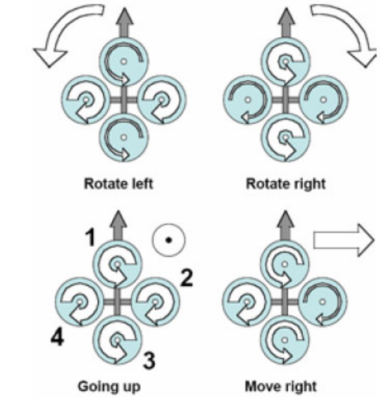$$ \underbrace{\begin{bmatrix}m\mathbb I & 0 \ 0 & \boldsymbol\Theta\end{bmatrix}}{\textbf M}\underbrace{\begin{bmatrix}\dot{\boldsymbol \nu} \ \dot{\boldsymbol \omega}\end{bmatrix}}}} + \underbrace{\begin{bmatrix}\boldsymbol \omega \times m \boldsymbol \nu \ \boldsymbol \omega\times \boldsymbol \Theta\boldsymbol \omega\end{bmatrix}{\textbf b} = \underbrace{\begin{bmatrix}\textbf F\\underbrace{ M} $$}}\end{bmatrix}}_{\boldsymbol \tau

\[ _{\mathcal B}\textbf F= \underbrace{\textbf C_{\mathcal{IB}}^\top ~_{\mathcal I}\begin{bmatrix}0\\0\\mg\end{bmatrix}}_{_{\mathcal B}\textbf F_G} + \underbrace{\sum_{i=1}^4 ~_{\mathcal B}\begin{bmatrix}0\\0\\-T_i\end{bmatrix}}_{_{\mathcal B}\textbf F_{Aero}} \]

\[ _{\mathcal B}M = \underbrace{_{\mathcal B}\begin{bmatrix}l(T_4-T_2)\\l(T_1-T_3)\\0\end{bmatrix}}_{_{\mathcal B}M_T}+ \underbrace{_{\mathcal B}\begin{bmatrix}0\\0\\ \sum_{i=1}^4 Q_i(-1)^i\end{bmatrix}}_{_{\mathcal B} Q} \]

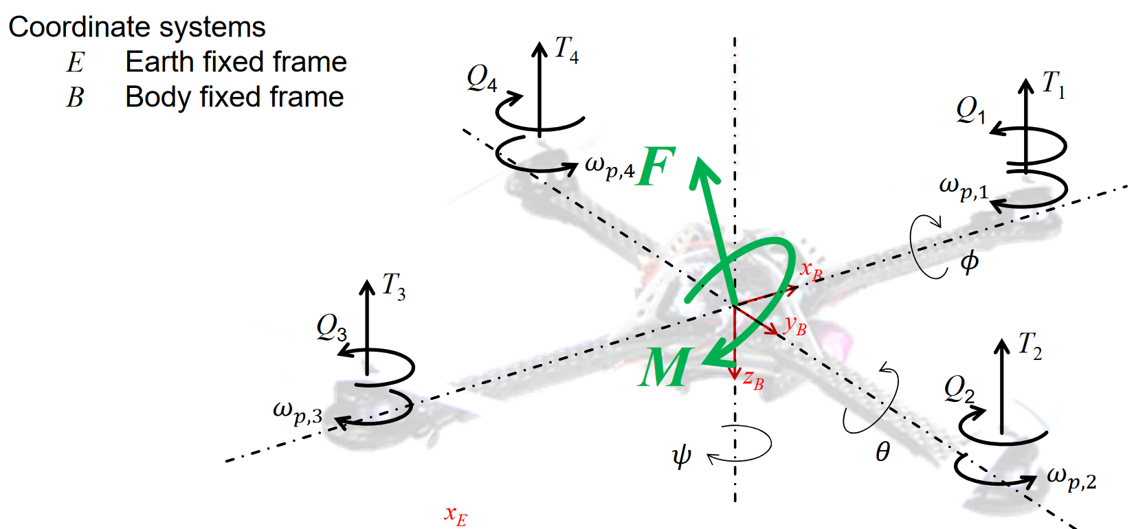
• \(T_i\) : Thrust force for propeller \(i\) , \(T_i = b\omega_{p,i}^2\) generate lift for keeping the rotorcraft in the air
• \(Q_i\) : Drag force of propeller \(i\) , \(Q_i=d\omega_{p,i}^2\) rotor drag
• \(_{\mathcal B}M_T\) : Thrust Induced moment, \(M_T = \begin{bmatrix}-\sin\theta\\\sin\phi\cos\theta\\\cos\phi \cos\theta\end{bmatrix}mg\)
• \(_{\mathcal B}Q\) : Drag torques/moment
• \(\textbf C_{\mathcal {IB}}\) : transition from earth frame to body frame ,
• \(_{\mathcal B}\boldsymbol \omega\) : Body Angular Velocity \(_{\mathcal B}\boldsymbol \omega =_{\mathcal B} \begin{bmatrix}p\\q\\r\end{bmatrix}=\begin{bmatrix}\dot \phi\\\dot \theta\\\dot \psi\end{bmatrix}\)
• \(\omega_{p,i }\) : Rotational Speed of Propeller \(i\)
• \(_{\mathcal B}\boldsymbol \nu\) : Basis Translation Velocity \(_{\mathcal B}\boldsymbol \nu = _{\mathcal B}\begin{bmatrix}u\\v\\w\end{bmatrix} = _{\mathcal B}\begin{bmatrix}\dot x\\\dot y \\\dot z\end{bmatrix}\)
• \(l\) : Distance of the propeller from the central of gravity

Control of Quadrotor

$$ \begin{array}{lr} \boldsymbol \Theta_{xx}\dot p = q\cdot r(\boldsymbol \Theta_{yy}-\boldsymbol \Theta_{zz}) + U_2 & (1) \

\boldsymbol \Theta_{yy}\dot q = r\cdot p(\boldsymbol \Theta_{zz}-\boldsymbol \Theta_{xx}) + U_3 & (2) \

\boldsymbol \Theta_{zz}\dot r = U_4 & (3) \

m\dot u = m(r\cdot v - q\cdot w )- \sin\theta~ mg & (4) \ m\dot v = m(p\cdot w - r\cdot u ) + \sin \phi \cos \theta ~ mg & (5) \ m\dot w = m(q\cdot u - p\cdot v) + \cos \phi \cos \theta ~ mg - U_1 & (6) \end{array} $$

\[ \begin{bmatrix}U_1\\U_2\\U_3\\U_4\end{bmatrix}= \underbrace{\begin{bmatrix}b&b&b&b\\ 0&-lb&0&lb\\ lb&0&-lb&0\\ -d&d&-d&d\end{bmatrix}}_{\textbf A} \begin{bmatrix}\omega_{p,1}^2\\\omega_{p,2}^2\\\omega_{p,3}^2\\\omega_{p,4}^2\end{bmatrix} \]

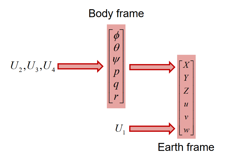
Equilibrium

\[_{\mathcal B}\boldsymbol \nu = \phi = \theta=\textbf 0\]

• \(_{\mathcal B} \dot{\boldsymbol \omega} = \boldsymbol \Theta^{-1}\begin{bmatrix}U_2&U_3&U_4\end{bmatrix}^\top\)

• \[ \begin{array}{l} U_1 = T^* \\ U_2 = (\phi^* - \phi)k_{p,roll}-\dot\phi k_{d,roll} \\ U_3 = (\theta^* - \theta)k_{p,pitch}-\dot\theta k_{d,pitch} \\ U_4 = (\psi^* - \psi)k_{p,yaw} - \dot \psi k_{d,yaw} \end{array} \]

Altitude Control

\[x=y=u=v=0\]

• \(\dot w = g- \frac{1}{m}\underbrace{\cos\phi\cos\theta ~U_1}_{T_z}\)
• \(T_z = -k_p(z^*-z)+k_d\dot z - mg\)

Position Control

\[_{\mathcal B}{\dot {\boldsymbol \nu}} = \frac{1}{m}\begin{bmatrix}T_x&T_y&T_z\end{bmatrix}^\top + \begin{bmatrix}0&0&g\end{bmatrix}^\top\]

Hexacopter

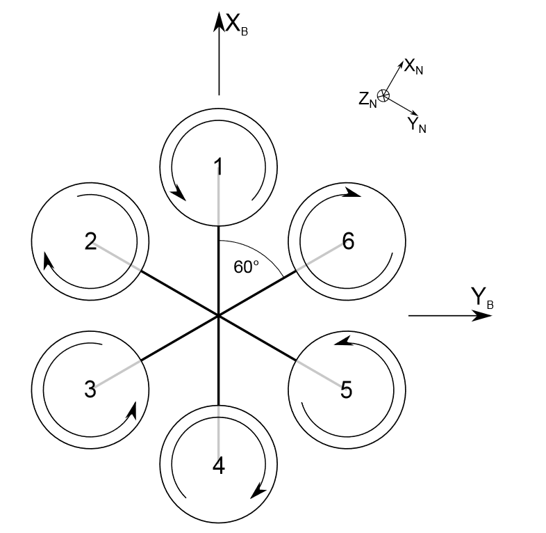
• \(\textbf C_{\mathcal{IB}}\)​ : rotation matrix from navigation to body frame
• \(\textbf p_i\) : poistion vector for propeller \(i\) , \(\textbf p_i = [l_{xi},l_{yi},0]^\top\)
• \(\textbf g\) : gravity \(\textbf g = \textbf C_{\mathcal{IB}}^\top [0,0,g]^\top\)
• \(\textbf T\) : thrust \(\textbf T = \sum_{i=1}^6[0,0,b\omega_{p,i}^2]\)
• \(\textbf M_Q\) : drag moment \(\textbf M_Q = \sum_{i=1}^6 [0,0,d\omega_{p,i}^2](-1)^{i+1}\)
• \(\textbf M_T\) : thrust induced moment \(\textbf M_T = \sum_{i=1}^6[0,0,b\omega_{p,i}^2]\times\textbf p_i\)

\[ \textbf A = \begin{pmatrix}b&b&b&b&b&b\\ bls_{30} & bl & bls_{30}& -bls_{30} & -bl & -bl s_{30}\\ -bl c_{30} & 0 & blc_{30} & blc_{30} & 0 & -blc_{30} \\ d& -d & d & -d & d & -d\end{pmatrix} \]

MAV Control

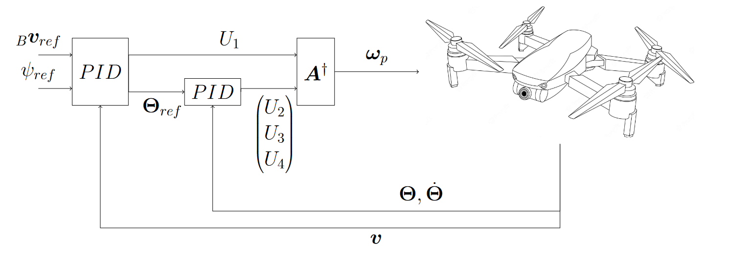
1. \(_{\mathcal B}\boldsymbol \omega_{ref} = \text{PID}(_{\mathcal B}\boldsymbol \nu_{ref},_{\mathcal B}\boldsymbol \nu)\)
2. \(U_1 = mg\\ \begin{bmatrix}U_2,U_3,U_4\end{bmatrix}^\top=\text{PID}(_{\mathcal B}\boldsymbol \omega_{ref},~_{\mathcal B}\boldsymbol \omega,~_{\mathcal B}\dot{\boldsymbol \omega})\)
3. \(\omega_p^2 = \textbf A^+ \begin{bmatrix}U_1&U_2&U_3&U_4\end{bmatrix}^\top\)

Propeller Aerodynamics

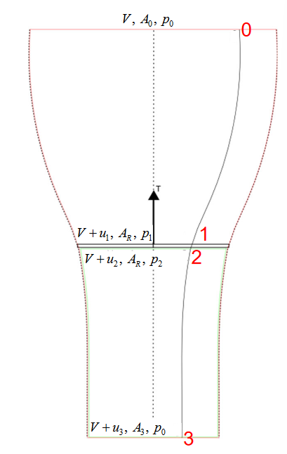
• \(u_1 = u_2\) : no change of speed across rotor/propeller disc
• \(\rho A_0 V = \rho A_R(V+u_1) = \rho A_R(V+u_2)=\rho A_3 u_3\) : change in pressure
• \(u_3 = 2u_1\) : far wake slipstream velocity is twice the induced velocity
• \(F_{\text{Thrust}} = \rho A_R(V+u_1)u_1\)
• \(P_{\text{Thrust}} = \frac{1}{2}\rho A_R(V+u_1)(2V + u_3) u_3\)
• Hover case : \(P = \frac{F^{3/2}_{\text{Thrust}}}{\sqrt{2\rho A_R}} = \frac{(mg)^{3/2}}{\sqrt{2\rho A_R}}\)

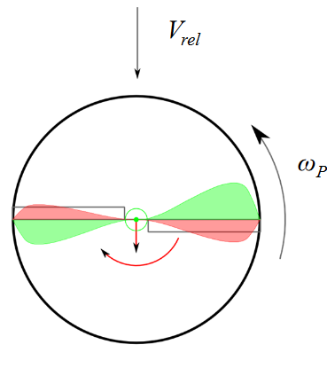
• \(T\) : Thrust force
• Aerodynamic force perpendicular to propeller plane
• \(|T|=\frac{\rho}{2}A_PC_T(\omega_PR_P)^2\)
• \(Q\) : Drag torque
• torque around rotor plane in the opposite direction of the propeller spinning direction
• \(|Q| =\frac{\rho}{2}A_PC_Q(\omega_PR_P)^2 R_P\)
• \(C_T\) , \(C_Q\) depend on blade pitch angle, reynolds number ...
• \(H\) : hub force
• opposite to horizontal flight direction \(V_H\)
• \(|H| = \frac{\rho}{2}A_PC_H(\omega_PR_P)^2\)
• \(R\) : Rolling moment
• around flight direction
• \(|R| = \frac{\rho}{2}A_PC_R(\omega_PR_P)^2R_P\)
• \(C_H\) ,\(C_R\) depend on the advance ratio \(\mu = \frac{V}{\omega_PR_P}\)

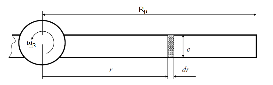
[BEMT]Blade Elemental and Momentum Theory : calculate forces for each element and sum them up

Fixed-Wing

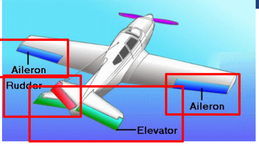
• Ailerons (rolling)
• Elevator (pitching)
• Rudder (yawing)

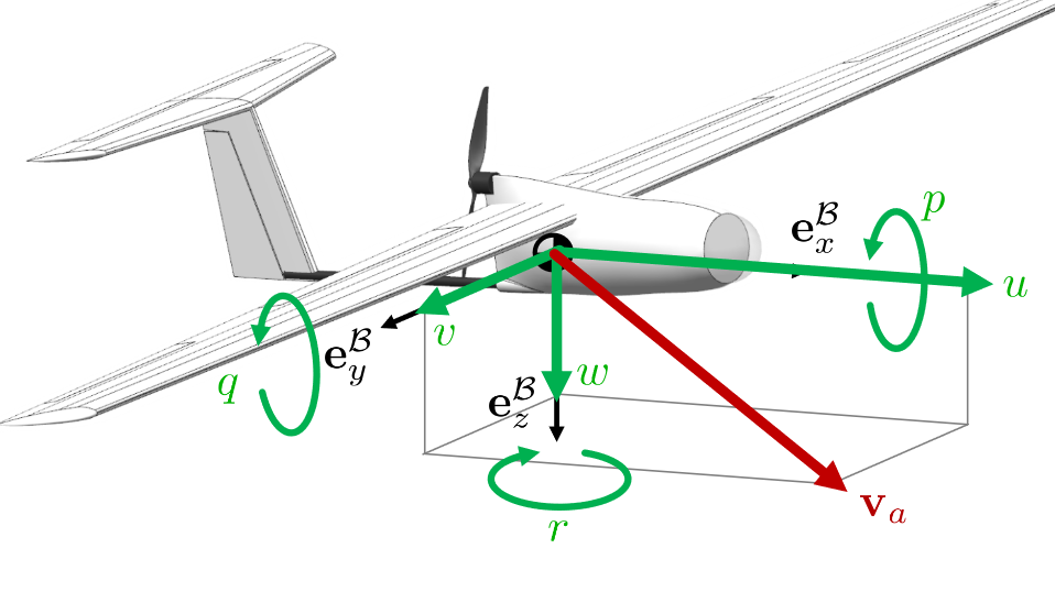
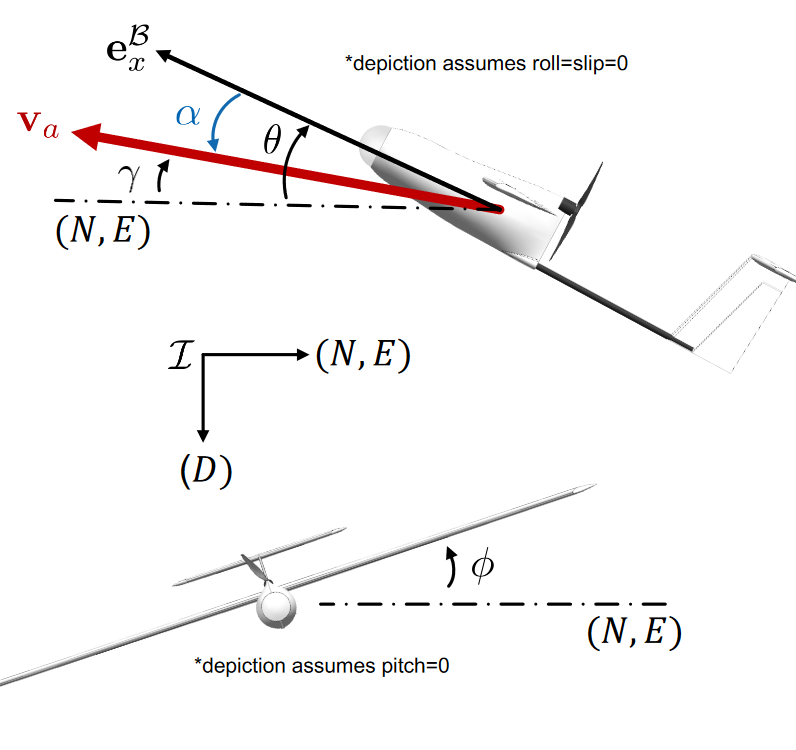
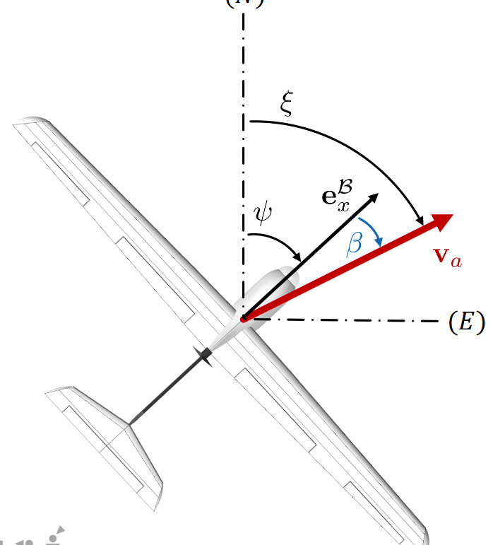
• \(\alpha\) : angle of attach \(\text{atan}(w/u)\)
• stall : \(\begin{cases}\alpha\uparrow \to c_L\uparrow & \alpha <\text{stall} \\ \alpha^\uparrow \to c_L\downarrow & \alpha > \text{stall}\end{cases}\) stall is not safe
• \(\beta\) : sideslip angle \(\beta = \asin(v/V)\)
• \(\theta\) : pitch angle
• \(\phi\) : roll angle , rotate about \(x\)-axis
• \(\psi\) : yaw angle
• \(\gamma\) : flight path angle, defined from horizon to \(\textbf v_a\)
• \(\xi\) : heading angle, defined from North to \(\textbf v_a\)
• \(\textbf v_w\) : wind velocity
• \(\textbf v\) : ground-based inertial velocity
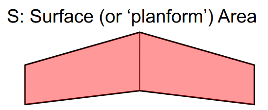
• \(L\) : Lift \(L=\frac{1}{2}\rho V^2 S{c_L}(\alpha)\) ,where \(S\) is the surface area
• \(D\) : Drag \(D=\frac{1}{2}\rho V^2 S{c_D}\), perpendicular to Lift, parallel to air velocity \(\textbf v_a\)
• minimum fuel for straight : \(\underset{\alpha}{\text{max}}\frac{c_L(\alpha)}{c_D(\alpha)}\)
• minimum fuel for circle : \(\underset{\alpha}{\text{max}}\frac{c_L(\alpha)^3}{c_D(\alpha)^2}\)
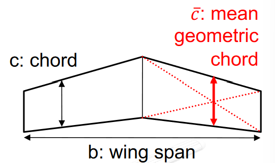
• \(L_m\) : rolling moment \(L_m = \frac{1}{2}\rho V^2 S{bc_l}\) , where \(b\) is the wing span
• \(M_m\) : pitching moment \(M_m = \frac{1}{2}\rho V^2 S{\bar cc_m}\), where \(c\) is the chord,
• \(N_m\) : yawing moment \(N_m = \frac{1}{2}\rho V^2 S{bc_n}\)

Steady Level Turning Flight

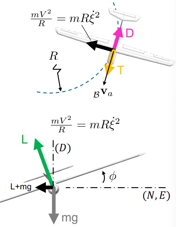
• steady : \(_{\mathcal B}\dot{\textbf v}_a = ~_{\mathcal B}\dot{\omega}=0\)
• level : \(\gamma = 0\)
• turning : \(\phi = \text{const}\) :

\[ \begin{array}{l} L\cos\phi = mg \\ L\sin \phi = m\frac{V^2}{R} = mR\dot\xi \\ D=T \end{array} \quad \rightarrow \quad \begin{array}{l} \dot{\xi} = \frac{g\tan\phi}{V} \\ L\propto \frac{1}{\cos\phi} \\ V\propto \sqrt{\frac{1}{\cos\phi}} \end{array} \]

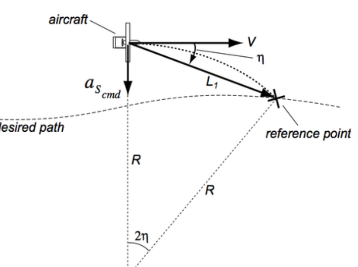
\(\mathcal L_1\) Guidance

$$ \begin{array}{l} a_s = \frac{V^2}{R} = 2\frac{V^2 \sin\eta}{L_1} \ \dot\phi \approx \dot\xi= \phi_d = \text{atan}\left(\frac{a_s}{g}\right) \end{array} $$

Total Energy Control System

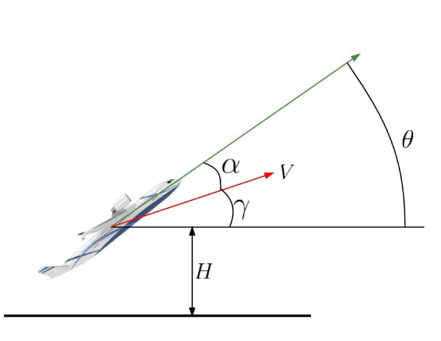
• \(\dot E_{spec} = \frac{\dot E_{tot}}{mgV}=\frac{\dot V}{g}+\sin\gamma\approx \frac{\dot V}{g}+\gamma\)
• \(\dot E_{dist} = \gamma - \frac{\dot V}{g}\)

Modeling for Control (Linearized Plant)

Longitudinal Plant

input : \(\Delta \delta_e, \Delta\delta_T\)

output : \(\Delta u, \Delta w, \Delta q,\Delta\theta\)

• Short Period Mode \(\mathbb C\) : \(\omega=5\text{rad}/s\)

  

  exchange between kinetic and potential energy: slow

• Phugoid Mode \(\mathbb C\) : \(\omega = 0.6~\text{rad}/s\)

  

  oscillation of angle of attack : fast

Lateral Plant

input : \(\Delta \delta_a, \Delta \delta_r\)

output : \(\Delta v,\Delta p, \Delta r, \Delta\phi,\Delta\psi\)

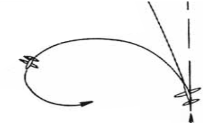
• Spiral Mode \(\mathbb R\): unstable

  

• Dutch Roll Mode \(\mathbb C\) : \(\omega = 5\text{rad}/s\)

  

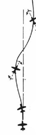
• Roll Subsidence \(\mathbb R\)

Statements

Kinematics

• : A homogeneous transformation \(T_{\mathcal {AB}}\) from frame \(\mathcal B\) to \(\mathcal A\) applied to a vector only changes its representation but not the underlying \(v\)
• : A rotation matrix \(C_{\mathcal {AB}}\) between from frame \(\mathcal B\) to \(\mathcal A\) applied to a vector only changes its representation but not the underlying \(v\)
• : A planar two-link robot arm has a unique solution to the inverse kinematic problem
• : For a planar two-link robot arm, the differential inverse kinematic algorithm always converges to the same solution irrespective of initial configuration
• : floating base in 3-dimensional space there exists a choice of generalized coordinates such that the analytical and geometric orientation Jacobian are equal

Dynamics

• : Given a perfect model, a robotic arm controlled by a PD controller with gravity compensation can achieve zero tracking error for any desired trajectory.
• : When choosing a unit quaternion as part of the generalized coordinates of a free-floating rigid body in 3D space, the mass matrix must have dimensions \(7\times 7\)

Legged Robot

• : For a bipedal system with two point feet on the ground, every torque command results in a unique acceleration
• : For a bipedal system with two point feet on the ground, every constraint consistent acceleration \(\dot u^∗_{consistent}\) is achieved by a unique torque command

Rotor Craft

• : A classic hexacopter (multi-rotor with 6 propellers) with all propellers spinning in the same plane is a fully actuated platform
• : The yaw motion for a quadcopter is controlled by the drag moment of the propeller
• : The attitude dynamics of a quadcopter can be stabilized by a proportional controller only
• : The hub force on a rotor in froward flight results mostly due to an imbalance of the lift forces on the advancing and the retreating blade.
• : BEMT can be used to model propeller characteristics, where momentum theory enables solving for induced velocities.
• : A swashplate has generally three degree of freedom . One to control the cyclic pitch and two to control the collective pitch.
• : A rotor in forward motion has a reverse flow region on the advancing blade
• : In a front-rear rotor configuration, the yaw motion is steered by differential drag torques of the rotors.
• : According to the momentum theory, the power consumption decrease to zero by increasing the disc area to infinity

Fixed Wing

• : The magnitude of the GPS velocity can be used directly as an airspeed measurement
• : The heading of a conventional aircraft is controlled primarily by the rudder
• : Wind disturbances are typically modeled/mitigated within the guidance- level loops of a fixed-wing autopilot
• : Minimum airspeed demand during a coordinated turn increases as the turning radius decreases, assuming constant angle of attach
• : in a coordinate turn, the sideslip force causes the needed centripetal acceleration