Sparse 路线:softmax + 跳过部分 (q,k) 对¶
更新日期:2026-04-26
核心原理:仍用 \(\text{softmax}(QK^\top) V\),但不让所有 query 看所有 K/V。用 mask(静态)或 indexer(动态)决定哪些 (q, k) 对参与 softmax。
跟 Full 路线 K/V 压缩相比:
- Full 压表示(K/V dim 变小)→ 信息密度高但仍全 attend
- Sparse 跳计算(部分 (q, k) 对置零)→ 计算量降但 attention 矩阵稀疏
主要变体一览:
| 变体 | 稀疏 pattern | 选择方式 | 复杂度 | 代表 |
|---|---|---|---|---|
| Sliding Window | 只看前 W 个 token | 静态 mask | \(O(N W)\) | Mistral 7B (W=4096) |
| Block Sparse | 块对角 + 全局 | 静态 mask | \(O(N \sqrt{N})\) | BigBird, Longformer |
| Strided / Dilated | 跳格子 | 静态 mask | \(O(N \log N)\) | Sparse Transformer |
| DSA (V3.2) | 每 query 选 top-k | 动态(lightning indexer) | \(O(N \cdot d_\text{idx} + k d_h)\) | DeepSeek-V3.2 |
| CSA (V4) | 序列 4× 压缩 + DSA | 动态 + 压缩 | \(O((N/m) d_\text{idx} + k d_h)\) | DeepSeek-V4 |
| Native Sparse Attn | 学习的 sparse pattern | 动态 | varies | DeepSeek NSA / Kimi K2 |
FlashAttention 严格说不是 sparse——它是 dense \(O(N^2)\) 计算的 IO-aware tiling 优化(fuse softmax + matmul,避免 attention matrix 写到 HBM)。混进 sparse 表只会让人误解,详见本文 §五 IO 优化章节。
一、为什么需要 Sparse Attention¶
1.1 Full Attention 的 O(n²) 代价¶
标准 Self-Attention 的核心运算:
\(\text{Attn}(Q,K,V) = \text{softmax}\!\left(\frac{QK^\top}{\sqrt{d_k}}\right) V\)
其中 \(Q, K, V \in \mathbb{R}^{n \times d}\),\(n\) 为序列长度,\(d\) 为头维度。
计算复杂度:\(QK^\top\) 的矩阵乘法为 \(O(n^2 d)\),softmax 为 \(O(n^2)\),乘 \(V\) 再一次 \(O(n^2 d)\)。总计 \(O(n^2 d)\) FLOPs per head per layer。
存储复杂度:注意力矩阵 \(S = QK^\top / \sqrt{d_k}\) 需要存储 \(n^2\) 个元素。
1.2 具体数字:128K context + 70B model¶
以 LLaMA-3 70B 为参考(\(H=64\), \(d_h=128\), \(L=80\) layers, GQA \(n_{kv}=8\)): 关键观察:
-
在 4K 时 FFN 计算远大于 Attention(compute-bound 在 FFN)。
-
在 128K 时 Attention 的 \(O(n^2)\) 开销反超 FFN,成为瓶颈。交叉点大约在 \(n \approx 8d_{model} \approx 65K\)。
-
128K 的注意力矩阵需要 2 TB 显存——任何硬件都无法存储;即使用 FlashAttention 不存储完整矩阵,计算量也是 4K 的 1024 倍。
1.3 瓶颈分解¶
二、Sparse Attention 全景¶
重要区分:FlashAttention 和 SageAttention 不改变注意力的数学语义(仍是全 \(O(n^2)\) attention),但通过硬件层面优化大幅加速。它们与 Sparse Attention 正交且可组合——例如 FlashAttention 已原生支持 Sliding Window mask。
三、Sliding Window Attention¶
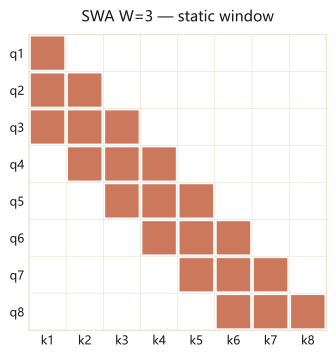
3.1 核心思想¶
每个 token \(i\) 只关注位置 \([i-w, i]\) 内的 token(causal 情况下只看左侧),\(w\) 为窗口大小。
\(\text{Attn}_i = \text{softmax}\!\left(\frac{q_i \cdot K_{[i-w:i]}^\top}{\sqrt{d_k}}\right) V_{[i-w:i]}\)
3.2 Mistral 的设计选择¶
Mistral 7B (Jiang et al., 2023) 采用 \(w=4096\) 的 sliding window,配合 32 层 Transformer。
有效感受野:第 \(l\) 层的 token 可通过逐层传递访问 \(l \times w\) 距离的信息。32 层 × 4096 窗口 = 理论上 131,072 token 的有效范围。
3.3 与 RoPE 的交互¶
RoPE 为位置 \(m\) 的向量施加旋转 \(R_{\Theta,m}\),使内积 \(\langle R_{\Theta,m} q, R_{\Theta,n} k \rangle\) 仅依赖相对位置 \(m-n\)。
在 Sliding Window 中:
-
窗口内 token 的相对位置 \(|m-n| \leq w\),RoPE 编码值在正常范围内。
-
窗口外 token 不参与计算,不存在 RoPE 外推问题。
-
多层传递的信息并非通过注意力分数的位置编码传递,而是通过隐状态向量——因此不受 RoPE 频率衰减影响。
3.4 KV Cache 节省¶
3.5 实现伪代码¶
class SlidingWindowAttention:
    def __init__(self, d_model, n_heads, n_kv_heads, window_size):
        self.window_size = window_size
        self.n_heads = n_heads
        self.n_kv_heads = n_kv_heads
        self.d_head = d_model // n_heads
        self.group_size = n_heads // n_kv_heads

        self.wq = Linear(d_model, n_heads * self.d_head)
        self.wk = Linear(d_model, n_kv_heads * self.d_head)
        self.wv = Linear(d_model, n_kv_heads * self.d_head)
        self.wo = Linear(n_heads * self.d_head, d_model)

    def forward(self, x, freqs_cis, kv_cache=None):
        B, S, _ = x.shape
        Q = self.wq(x).view(B, S, self.n_heads, self.d_head)
        K = self.wk(x).view(B, S, self.n_kv_heads, self.d_head)
        V = self.wv(x).view(B, S, self.n_kv_heads, self.d_head)

        Q, K = apply_rotary_emb(Q, K, freqs_cis)

        if kv_cache is not None:
            K, V = kv_cache.update(K, V)
            K, V = kv_cache.get_last(self.window_size)  # 只取最近 w 个

        K = K.repeat_interleave(self.group_size, dim=2)
        V = V.repeat_interleave(self.group_size, dim=2)

        scores = torch.einsum('bshd,bthd->bhst', Q, K) / math.sqrt(self.d_head)

        mask = build_sliding_window_mask(S, K.shape[1], self.window_size)
        scores = scores.masked_fill(~mask, float('-inf'))

        attn = F.softmax(scores, dim=-1)
        out = torch.einsum('bhst,bthd->bshd', attn, V)
        return self.wo(out.reshape(B, S, -1))


class RollingKVCache:
    def __init__(self, max_size, n_kv_heads, d_head):
        self.max_size = max_size
        self.buffer_k = torch.zeros(1, max_size, n_kv_heads, d_head)
        self.buffer_v = torch.zeros(1, max_size, n_kv_heads, d_head)
        self.pos = 0

    def update(self, k_new, v_new):
        seq_len = k_new.shape[1]
        indices = (torch.arange(seq_len) + self.pos) % self.max_size
        self.buffer_k[:, indices] = k_new
        self.buffer_v[:, indices] = v_new
        self.pos = (self.pos + seq_len) % self.max_size
        return self.buffer_k, self.buffer_v

    def get_last(self, window_size):
        w = min(window_size, self.max_size)
        indices = [(self.pos - 1 - i) % self.max_size for i in range(w)]
        indices.reverse()
        return self.buffer_k[:, indices], self.buffer_v[:, indices]
四、DSA / CSA — 动态 top-k 选择(DeepSeek V3.2 / V4)¶
SWA / BigBird 都是静态 mask(compile-time 决定哪些 (q, k) 对算)。DSA / CSA 是动态选择——每个 query 由学习的 indexer 在 runtime 选 top-k 个最相关的 KV。这俩跟 MLA 共生用于 frontier,是 §三 静态 sparse 的进化版。
4.1 DSA (DeepSeek Sparse Attention)¶
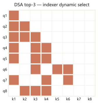
参考 DeepSeek-V3.2-Exp HF(2025-12)。
每个 query 不 attend 全部 KV,经一个 lightning indexer 选 top-k 个 KV 块。\(O(N^2) \to O(N \cdot k)\)(attend 部分),但 indexer 仍 \(O(N)\) per query——所以是 sub-quadratic 不是 linear。
class DSA(nn.Module):
    """简化版 DeepSeek Sparse Attention. 基于 MLA, 加 lightning indexer 选 top-k."""
    def __init__(self, d_model, n_heads, d_h, d_c, top_k=64):
        super().__init__()
        self.mla = MLA(d_model, n_heads, d_h, d_c)
        self.top_k = top_k
        # lightning indexer: 轻量打分网络(低秩 → 速度快)
        self.indexer_q = nn.Linear(d_model, d_c)
        self.indexer_k = nn.Linear(d_c, d_c)            # 作用在 c_kv 上

    def forward(self, x, c_kv_cache):
        B, S, _ = x.shape
        # 1. lightning indexer 给所有 (q, k) 打分
        q_idx = self.indexer_q(x)                       # [B, S, d_c]
        k_idx = self.indexer_k(c_kv_cache)              # [B, T, d_c]
        scores = q_idx @ k_idx.transpose(-2, -1)        # [B, S, T]   ← 这一步仍 O(N²)
        topk_idx = scores.topk(self.top_k, dim=-1).indices  # [B, S, top_k]

        # 2. 收集 top-k 对应的 c_kv(gather)
        c_kv_topk = torch.gather(
            c_kv_cache.unsqueeze(1).expand(-1, S, -1, -1),
            2,
            topk_idx.unsqueeze(-1).expand(-1, -1, -1, c_kv_cache.size(-1)),
        )  # [B, S, top_k, d_c]

        # 3. 在 top-k 子集上跑 MLA attention
        return self.mla.attend_subset(x, c_kv_topk)
为什么是 Sparse 而不是 Full:第 3 步只 attend 到 top-k 个 KV,不是全部 —— 这是 sparse selection 的定义。lightning indexer 用低秩投影让步骤 1 比 full softmax attention 便宜很多(\(d_\text{idx} \ll H d_h\)),但 selection 本身仍是 sparse 操作。
4.2 CSA (Compressed Sparse Attention)¶
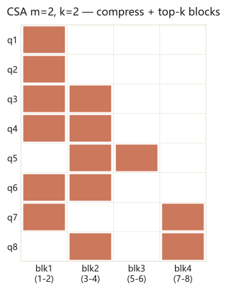
DSA 把 indexer 跑在原始序列上仍 \(O(N)\) per query。CSA 先沿序列维 4× 压缩,indexer 跑在压缩后的 \(N/m\) 个块上 → 进一步 sub-linear。
class CSA(nn.Module):
    """每 m=4 个 KV 学习压成 1 个块,再 DSA 选 top-k 块。"""
    def __init__(self, d_model, d_c, m=4, top_k=64):
        super().__init__()
        self.m = m
        # softmax-gated pooling: 块内 m 个 token 加权合成 1 个
        self.gate = nn.Linear(d_c, m)
        self.pos_bias = nn.Parameter(torch.zeros(m, d_c))
        self.dsa = DSA(d_model, n_heads=128, d_h=128, d_c=d_c, top_k=top_k)

    def compress(self, c_kv):
        B, T, d = c_kv.shape
        T_blocks = T // self.m
        c_kv_blocks = c_kv[:, :T_blocks * self.m].reshape(B, T_blocks, self.m, d)
        gate_logits = self.gate(c_kv_blocks).softmax(dim=-2)
        weighted = c_kv_blocks + self.pos_bias
        compressed = (gate_logits.unsqueeze(-1) * weighted.unsqueeze(-2)).sum(-2).mean(-2)
        return compressed                                       # [B, T/m, d]

    def forward(self, x, c_kv_cache):
        compressed = self.compress(c_kv_cache)                  # 4× 压缩 → N/4 块
        return self.dsa(x, compressed)                          # 在压缩块上 DSA top-k
4.3 V4 = HCA (Full) + CSA (Sparse) 双路径¶
DeepSeek-V4 真实架构 = CSA 看局部细 + HCA 看全局粗,两路并行输出叠加。1M ctx 实测:
- KV cache: BF16 GQA8 baseline 的 2%(即 50× 压缩)
- 单 token inference FLOPs: V3.2 的 27%
- 整体相比 V3.2:−73% FLOPs + −90% KV memory
V4 同时跨了 Full(HCA)和 Sparse(CSA)两条路线——同 layer 内 hybrid,是 frontier 罕见的"细粒度+粗粒度"双引擎设计。HCA 在 full.md 有详细介绍。
五、SageAttention¶
5.1 核心观察¶
Attention score 矩阵 \(S = QK^\top / \sqrt{d_k}\) 在 softmax 之前是平滑的——相邻元素差异小,整体分布近似正态。这意味着 对 Q 和 K 做 INT8 量化产生的误差在 softmax 后被大幅压缩。
直觉:如果 \(S_{ij}\) 和 \(\hat{S}_{ij}\)(量化后的近似值)差距 \(\epsilon\),softmax 的输出差距约为 \(O(\epsilon \cdot \sigma^2)\),其中 \(\sigma^2\) 是 attention score 的方差。对于平滑分布 \(\sigma^2\) 小,误差被抑制。
5.2 SageAttention v1¶
核心方法:
-
Per-warp 量化 Q, K → INT8:对每个 warp 负责的 tile 独立计算 scale,最大化量化精度。
-
INT8 Tensor Core 计算 \(QK^\top\):利用 INT8 GEMM 的 2x 吞吐量(相比 FP16)。
-
反量化回 FP16 → softmax → FP16 matmul with V:V 保持 FP16 精度。
def sage_attention_v1(Q, K, V, block_m=128, block_n=64):
    N, d = Q.shape
    O = torch.zeros_like(V)

    for i in range(0, N, block_m):
        q_block = Q[i:i+block_m]
        q_scale = q_block.abs().amax(dim=-1, keepdim=True) / 127.0
        q_int8 = (q_block / q_scale).round().to(torch.int8)

        row_max = torch.full((block_m,), float('-inf'))
        row_sum = torch.zeros(block_m)
        acc = torch.zeros(block_m, d)

        for j in range(0, N, block_n):
            k_block = K[j:j+block_n]
            k_scale = k_block.abs().amax(dim=-1, keepdim=True) / 127.0
            k_int8 = (k_block / k_scale).round().to(torch.int8)

            s_int32 = q_int8 @ k_int8.T  # INT8 Tensor Core
            s_fp16 = s_int32.float()  (q_scale  k_scale.T) / math.sqrt(d)

            new_max = torch.maximum(row_max, s_fp16.max(dim=-1).values)
            exp_old = torch.exp(row_max - new_max)
            p = torch.exp(s_fp16 - new_max.unsqueeze(-1))

            row_sum = row_sum * exp_old + p.sum(dim=-1)
            acc = acc * exp_old.unsqueeze(-1) + p @ V[j:j+block_n].float()
            row_max = new_max

        O[i:i+block_m] = (acc / row_sum.unsqueeze(-1)).half()

    return O
5.3 SageAttention v2¶
5.4 性能数据¶
精度影响(LLaMA-2 7B, WikiText-2 perplexity): 实践意义:SageAttention 是目前推理加速最 "plug-and-play" 的方案——不改模型结构、不改训练流程,只替换 attention kernel 即可获得 2x+ 加速。与 FlashAttention 正交,实际上 SageAttention 内部使用了 FlashAttention 相同的 online softmax tiling 策略。
六、Sparse 与其他路线的关系¶
Linear / RNN 路线本身是另一个独立家族,详见 linear.md。Sparse + Linear hybrid 的具体配比方案(Jamba / Nemotron / Kimi Linear / MiniMax M1)在 attention/index.md §五 Hybrid 设计 一处统一讲,避免重复。
本节只点出互补关系:
- Sparse(此处)= 保留 softmax,跳过部分 (q,k) 对,牺牲信息可达性换计算量
- Linear(linear.md)= 砍 softmax + 固定 state 矩阵,牺牲精确召回换 KV 常数
两者在 frontier 经常同时使用(如 MiniMax-M1 = Lightning Linear + softmax MHA hybrid,softmax 层本身可以再加 Sliding Window mask 进一步省)。
选型决策、跨路线 trade-off、各家 hybrid 比例 → attention/index.md §七 选型决策
七、追问延伸¶
| 问题 | 分析 | 深度方向 |
|---|---|---|
| Sliding Window 会导致远距离信息完全丢失吗? | 不会。信息通过多层隐状态传递,但会逐层衰减——类似 SSM 的指数遗忘。经验上 LLaMA-3 128K 在 NIAH 任务表现良好,说明 full attention 的多层传递优于 sliding window | 量化分析多层传递的信息保留率;与 SSM 的遗忘曲线对比 |
| SageAttention 能用于训练吗? | 目前主要用于推理。训练时 backward 需要对量化操作做 STE(Straight-Through Estimator),误差会累积。但 FP8 训练(如 DeepSeek-V3)已经验证了低精度 attention 训练的可行性 | |
| FlashAttention 支持哪些稀疏模式? | FA⅔ 原生支持 causal mask 和 sliding window mask。自定义稀疏模式需要 FlexAttention (PyTorch 2.5+) 或 Triton 手写 | FlexAttention 的 block mask API 允许用 Python 定义任意稀疏模式并 JIT 编译为高效 kernel |
| 为什么 Reformer (LSH) 实际很少被用? | LSH 的常数因子大,实际速度在 \(n < 64K\) 时不比 FlashAttention 快;多轮 hash 的准确率-速度 tradeoff 不如固定模式 sliding window 可控;GPU 不擅长动态稀疏 | 固定模式 vs 数据依赖模式的工程 tradeoff |
| Native Sparse Attention (NSA, DeepSeek) 是什么? | DeepSeek 提出的 learned sparse attention:模型学习每个头/层的最优稀疏模式,而非手工设定。训练时 full attention + Gumbel-softmax 选择;推理时固化为静态模式 | NSA (DeepSeek, 2025):结合 compression token + sliding window + selection token 三种模式 |
| Ring Attention 与 Sparse 的关系? | Ring Attention 是序列并行策略,不改变注意力模式。可与 Sparse 组合:每个设备只需发送/接收窗口内的 KV block,通信量从 \(O(n)\) 降为 \(O(w)\) |
参考文献¶
-
Child, R., Gray, S., Radford, A., & Sutskever, I. (2019). Generating Long Sequences with Sparse Transformers. arXiv:1904.10509
-
Kitaev, N., Kaiser, Ł., & Levine, A. (2020). Reformer: The Efficient Transformer. arXiv:2001.04451
-
Beltagy, I., Peters, M. E., & Cohan, A. (2020). Longformer: The Long-Document Transformer. arXiv:2004.05150
-
Zaheer, M., et al. (2020). Big Bird: Transformers for Longer Sequences. arXiv:2007.14062
-
Dao, T., Fu, D. Y., Ermon, S., Rudra, A., & Ré, C. (2022). FlashAttention: Fast and Memory-Efficient Exact Attention with IO-Awareness. arXiv:2205.14135
-
Dao, T. (2023). FlashAttention-2: Faster Attention with Better Parallelism and Work Partitioning. arXiv:2307.08691
-
Shah, J., Bikshandi, G., Zhang, Y., Thakkar, V., Ramani, P., & Dao, T. (2024). FlashAttention-3: Fast and Accurate Attention with Asynchrony and Low-precision. arXiv:2407.08608
-
Jiang, A. Q., et al. (2023). Mistral 7B. arXiv:2310.06825
-
Zhang, J., et al. (2024). SageAttention: Accurate 8-Bit Attention for Plug-and-play Inference Acceleration. arXiv:2410.02367
-
Zhang, J., et al. (2024). SageAttention2: Efficient Attention with Thorough Outlier Smoothing and Per-thread INT4 Quantization. arXiv:2411.10958
-
Lieber, O., et al. (2024). Jamba: A Hybrid Transformer-Mamba Language Model. arXiv:2403.19887
-
DeepSeek-AI. (2025). Native Sparse Attention: Hardware-Aligned and Natively Trainable Sparse Attention. arXiv:2502.11089
-
Milakov, M. & Gimelshein, N. (2018). Online normalizer calculation for softmax. arXiv:1805.02867
↑ 上级 · A2 注意力机制全景