Probabilitisc Artificial Intelligence¶

professor: Andreas Krause¶

1. Gaussian¶

\[ \mathcal N (x|\mu,\sigma) = \frac{1}{(2\pi)^{\frac{n}{2}}\sqrt{|\Sigma|}}exp(-\frac{1}{2}(x-\mu)^T\Sigma^{-1}(x-\mu)) \]

among all distributions over the real numbers with known mean and variance, Gaussian distribution has the maixmum entropy.

1.0. Deduce¶

suppose the gaussian distribution is $f(x)$

Assumption 1:distribution is isotropic, so we consider it in 2-D. $$ f(x)f(y) = f(\sqrt{x^2+y2})f(0) $$ Then, let's divide each side by $f(0)^2$. $$ \frac{f(x)}{f(0)}\frac{f(y)}{f(0)} = \frac{f(\sqrt{x^2+y2})}{f(0)} $$ Then, apply $ln$ to transform multiply to addition. $$ ln(\frac{f(x)}{f(0)}) + ln(\frac{f(y)}{f(0)}) = ln(\frac{f(\sqrt{x^2+y2})}{f(0)}) $$ To make it easier, we denote $g(x) = ln(\frac{f(x)}{f(0)})$. $$ g(x)+g(y) = g(\sqrt{x^2+y2}) $$ Now, it's easy to figure out the solution of $g(x)$. ($c$ is a constant number here) $$ g(x) = cx^2 $$ So we could get the expression of $f(x)$. $$ f(x) = f(0)e^{cx2} $$ Assumption 2: The integral of $f(x)$ is $1$. $$ \int_{-\infin}^{\infin}f(x) dx = 1 $$ Also put it int 2-D. $$ \begin{aligned} (\int_{-\infin}^{{\infin}f(x)dx)}2 &=\int_{-\infin}^{{\infin}\int_{-\infin}}f(x)f(y)dxdy \ &=\int_{-\infin}^{{\infin}\int_{-\infin}}f(0)^2e{c(x^2+y2)}dxdy \ &=\int_{0}^{{\infin}\int_{0}}f(0)^2erd\theta dr \ &=2\pi f(0)^2 (\frac{e^{cr2}}{2c})|{r=0}^{r=\infin} \ &=-\frac{\pi f(0)^2}{c} = 1 \end{aligned} $$ So we can represent $f(0)$ using $c, c<0$ $$ f(x) = \sqrt{\frac{-c}{\pi}}e^{cx2} $$ Now we got a $n$ sample data ${x_1, x_2,\cdots, x_n}$ from distribution $f(x)$. And we can calculate their expectation ($\mu$) and standard deviation ($\sigma$). $$ \begin{aligned} \mu &= \sum^n x_i \ \sigma & =\sqrt{\frac{1}{n}\sum_{i=1}^n(x_i-\mu)2} \end{aligned} $$ To represent $c$ with $\mu,\sigma$, we use the Maximum likelihood estimate $$ \begin{aligned} &L(x) = \prod_{i=1}^nf(x-x_i) \ &\Rightarrow ln(L(x)) = \sum_{i=1}^nln(f(x-x_i)) \ &\Rightarrow \begin{cases} \frac{\partial ln(L(x))}{\partial x} = 0 \ \frac{\partial ln(L(x))}{\partial c} = 0 \end{cases} \ &\Rightarrow \begin{cases} x = \mu \ c = -\frac{1}{2\sigma^2} \end{cases} \end{aligned} $$ So we could get the full expression of $f(x)$ which is corresponding to $\mathcal N(0, \sigma)$. $$ f(x) = \frac{1}{\sqrt{2\pi}\sigma}exp(-\frac{x^2}{2\sigma2}) $$ Intuitively, we could get the representation of $\mathcal N(\mu, \sigma)$. $$ f(x) = \frac{1}{\sqrt{2\pi}\sigma}exp(-\frac{(x-\mu)^2}{2\sigma2}) $$ As higher dimension, $\mu,x\in \mathbb R^d$ becomes a vector. For the most simple case, each element in $x$ is orthogonal. Then $\sigma\in \mathbb R^d$ is also a vector. $$ f(x) = \frac{1}{(\sqrt{2\pi})^{d\sigma}exp(-\frac{(x-\mu)}T(x-\mu)}{2\sigma^2}) $$ But normally, each element of $x$ is not orthogonal. So consider a transformation $$ y = \frac{A(x-\mu)}{\sigma} $$ Then we could get the normal representation of gaussian distribution. We denote $\Sigma = \frac{\sigma^2}{A^TA}$ $$ \begin{aligned} f(y) &= \frac{|A|}{(\sqrt{2\pi})^{d\sigma}exp(-\frac{(x-\mu)}TA^{TA(x-\mu)}{2\sigma}2}) \ &= \frac{1}{(\sqrt{2\pi})^d |\Sigma|^{{\frac{1}{2}}}exp(\frac{1}{2}(x-\mu)}T\Sigma^{-1}(x-\mu)) \end{aligned} $$

1.1. $p(\mathcal N|\mathcal N)$¶

suppose $X_A, X_B$ are disjoint subsets from $X\sim \mathcal N(\mu_V,\Sigma_{VV})$

then $p(X_A|X_B=x_B) = \mathcal N(\mu_{A|B},\Sigma_{A|B})$ $$ \begin{aligned} \mu_{A|B} &= \mu_A + \Sigma_{AB}\Sigma_{BB}^{-1}(x_B - \mu_B) \ \Sigma_{A|B} &= \Sigma_{AA} - \Sigma_{AB}\Sigma_{BB}^{-1}\Sigma_{BA} \end{aligned} $$

1.2. $p(M\mathcal N)$¶

suppose $X\sim \mathcal N (\mu_X,\Sigma_{XX})$, and matrix $M\in \mathbb R^{m\times d}$.

then $Y = MX \sim \mathcal N(\mu_Y,\Sigma_YY)$ $$ \begin{aligned} \mu_Y &= M\mu_X\ \Sigma_{YY} &= M^T\Sigma_{XX}M \end{aligned} $$

1.3. $p(\mathcal N + \mathcal N)$¶

suppose $X\sim\mathcal N(\mu_X,\Sigma_{XX})$, and $X'\sim \mathcal N(\mu_{X'},\Sigma_{X'X'})$

then $Y= X+X'\sim \mathcal N(\mu_Y,\Sigma_{YY})$ $$ \begin{aligned} \mu_{Y} &= \mu_X + \mu_{X'}\ \Sigma_{YY} &= \Sigma_{X} + \Sigma_{X'} \end{aligned} $$

1.4. $p(\mathcal N\mathcal N)$¶

suppose $X\sim \mathcal N(\mu_X,\Sigma_{XX})$, and $X'\sim\mathcal N(\mu_{X'},\Sigma_{X'X'})$

then $Y = XX'\sim \mathcal N(\mu_Y,\Sigma_{YY})$ $$ \begin{aligned} \Sigma_{YY}&= (\Sigma_{XX}^{{-1}+\Sigma_{X'X'}} \ \mu_{Y} &= \Sigma_{YY}\Sigma_{XX}^{-1}\mu_X + \Sigma_{YY}\Sigma_{X'X'}^{-1}\mu_{X'} \end{aligned} $$ if })^{-1$X'\sim\mathcal N(0, I)$ $$ \begin{aligned} \Sigma_{YY} &= (\Sigma_{XX}^{-1}+I) \ \mu_{Y} &= \Sigma_{YY}\Sigma_{XX}^{-1}\mu_x \end{aligned} $$

2. Probability¶

Mean¶

\[ \mathbb E[x] = \frac{1}{n}\sum_{i=1}^n x_i \]

Variance¶

\[ \mathbb Var[x] = \mathbb E[x^2] - \mathbb E[x]^2 \]

Covariance $$ Cov[x,y] = \mathbb E[xy] - \mathbb E[x]\mathbb E[y] $$

\[ \mathbb Var[x-y] = \mathbb Var[x] + \mathbb Var[y] - 2Cov[x,y] \]

Max Likelihood Estimation (MLE)¶

\[ \hat \theta = argmax_{\theta}P(X_{1:n}|\theta) \]

sometimes will add $l_2$ norm which is $\Vert \cdot\Vert_2$ for vector and $\Vert \cdot \Vert_F$ for matrix

Max a priority(MAP)¶

\[ \hat \theta = argmax_\theta(X_{1:n}|\theta,X') \]

KL-Divergence¶

\[ D_{KL}(p\Vert q) = \int p(x)log\frac{p(x)}{q(x)}dx \]

$D_{KL}(p\Vert q)$ : mode averaging
$D_{KL}(q||p)$ : mode seeking, given $p \sim\mathcal N\left(0, \left[\begin{matrix}\sigma_1^2 & 0 \\ 0 &\sigma_2^2\end{matrix}\right]\right)$ , $\sigma_q^2 = \frac{2}{\frac{1}{\sigma_1^2}+\frac{1}{\sigma_2^2}}$
$D_{KL}(q||p)$ is well defined if $q$ is a subset of $p$

$\Gamma $ distribution¶

\[ \begin{aligned} \Gamma(x;\alpha,\beta) &= \frac{\beta^\alpha}{\Gamma(\alpha)}x^{\alpha-1}e^{-\beta x}\\ \mathbb E[\Gamma(x;\alpha,\beta)] &= \frac{\alpha}{\beta}\\ \mathbb Var[\Gamma(x;\alpha,\beta)] &= \frac{\alpha}{\beta^2} \end{aligned} \]

$\Beta$ distribution¶

\[ \begin{aligned} \Beta(x;\alpha,\beta) &= \frac{x^{\alpha-1}(1-x)^{\beta-1}}{\Beta(\alpha,\beta)} = \frac{\Gamma(\alpha)\Gamma(\beta)}{\Gamma(\alpha+\beta)}\\ \mathbb E[\Beta(x;\alpha,\beta)] &=\frac{\alpha}{\alpha+\beta}\\ \mathbb Var[\Beta(x;\alpha,\beta)] &= \frac{\alpha\beta}{(\alpha+\beta)^2(\alpha+\beta+1)} \end{aligned} \]

Bernoulli distribution¶

\[ \begin{aligned} Bernoulli(x;p) &= p^x(1-p)^{1-x}\\ \mathbb E[Bernoulli(x;p)] &= p\\ \mathbb Var[Bernoulli(x;p)] &= p(1-p) \end{aligned} \]

Poisson distribution¶

\[ \begin{aligned} Pr(x;\lambda) &= \frac{\lambda^k e^{-\lambda}}{k!}\\ \mathbb E[Pr(x;\lambda)] &= \lambda\\ \mathbb Var[Pr(x;\lambda)] &= \lambda\\ \end{aligned} \]

3. Bayesian Linear Regression¶

Assume

dataset $X = \{x_1,\cdots x_m\} ~ Y = \{y_1,\cdots y_m\}$

prior

$f(x_i) = x_i^T w$
$y_i = f(x_i) + \epsilon_i ~ \epsilon_i\sim\mathcal N(0,\sigma_n^2)$
$w\sim \mathcal N(0, \sigma_p^2)$

Then $$ \begin{aligned} P(w|Y,X) &= \mathcal N(\mu,\Sigma)\ \mu &= \frac{1}{\sigma_n^2}\Sigma X^TY\ \Sigma &= \left(\frac{1}{\sigma_n^2}XTX + \frac{1}{\sigma_p^2}I\right)\ f(x^)&\sim \mathcal N({x^*}T\mu, {x^*}T\Sigma{x^}) \end{aligned} $$

online¶

\[ \begin{aligned} X^\top X &= \sum_{i=1}^t x_i^\top x_i &\Rightarrow X_{new}X_{new}^\top &= X^\top X+x_{t+1}x_{t+1}^\top \\ X^\top Y &= \sum_{i=1}^t y_ix_i &\Rightarrow X_{new}^\top Y_{new} &= X^\top Y+ y_{t+1}x_{t+1} \end{aligned} \]

fast¶

reduce from $\mathcal O(d^3)$ to $\mathcal O(d^2)$

\[ (A+xx^\top)^{-1} = A^{-1} - \frac{(A^{-1}x)(A^{-1}x)^T}{1+x^\top A^{-1}x} \]

\[ (X_{new}^\top X_{new} + \sigma_n^2 I )^{-1} = (\underset{A}{\underbrace{X^\top X + \sigma_n^2}} + x_{t+1}x_{t+1}^\top)^{-1} \]

4. Gaussian Process¶

closed formulae for Bayesian posterior update exist

kernel¶

symmetric
semi definite

RBF Kernel¶

\[ k(u,v) = \sigma_F^2 exp\left(-\frac{(u-v)^2}{2l^2}\right) \]

$l$ length scale control the distance of data,
$\sigma_F$ output scale control the magnitude
$\underset{l\rightarrow 0}{lim}~k(u,v) = \sigma_F^2\delta(u-v)$
posterior variance: $\underset{l\rightarrow 0}{lim}~k'(x,x) = k(x,x) - k_{xX}(K_{XX}+\sigma_n^2 I)^{-1}k_{xX}^\top = \frac{\sigma_F^2\sigma^2}{\sigma_F^2 + \sigma^2}$

Assume

dataset $X = \{x_1,\cdots x_m\} ~ Y = \{y_1,\cdots y_m\}$

prior

$f \sim GP(\mu, k)$
$y_i = f(x_i) + \epsilon_i ~ \epsilon_i\sim\mathcal N(0,\sigma_n^2)$

Then $$ \begin{aligned} &P(f|X,Y)\sim GP(f;\mu',k') \ \mu'{x^} &= \mu_{x^} + K{x^{*X}(K_{XX}+\sigma_n}2I)^{-1}Y \ k'{x^*x} &= K_{x^*x} - K{x^*X}T(K_{XX}+\sigma_n^2I)K_{x^X} \end{aligned} $$ *Especially for Linear Kernel

$K(x,x') = \lambda x^Tx$ equals to BLR with $\lambda = \sigma_p^2$

Woodbury push-through $$ U(VU+I)^{-1} = (UV+I)^{-1}U $$

Fast GPS¶

\[ k(x,x') \approx \phi(x)^T \phi(x') \quad\phi(x)\sim \mathbb R^m \]

computational cost : $O(nm^2 + m^3)$

Fourier Features¶

\[ k(x,x') \approx k(x-x') \\ \Rightarrow k(x-x') = \int_{\mathbb R^d} p(\omega)e^{j\omega^T(x-x')}dw \]

Bochner Theorem : $p(\omega)\geq0 \Rightarrow k\geq 0$

Inducing points¶

Subset of Regressors(SoR) : $q_{SOR}(f|u)=\mathcal N(K_{f,u}K_{u,u}u,0) \approx \mathcal N(K_{f,u}K_{u,u}^{-1}u,K_{f,f}-Q_{f,f})$

Fully independent training conditional (FITC) : $q_{FIFC}(f|u)=\mathcal N(K_{f,u}K_{u,u}u,diag(K_{f,f-Q_{f,f}})) \approx \mathcal N(K_{f,u}K_{u,u}^{-1}u,K_{f,f}-Q_{f,f})$

optimize hyperparameters via maximizing the marginal likelihood

computational cost : $O(n^3)$ ($\because K_{u,u}^{-1}$)

Kalman Filter¶

\[ \begin{aligned} x_{t+1} &= F_tx_{t} + \Sigma_{x,t} \\ y_t &= H_t x^t + \Sigma_y \end{aligned} \]

predict $$ \hat x_{t+1} = F_t x_t \ \hat \Sigma_{x,t+1} = H_t \Sigma_{x,t}H_t^\top + \Sigma_{d_t} $$ correct $$ \begin{aligned} K_{t+1} &= \Sigma_{x,t}H_t^\top (H_t\hat \Sigma_{x,t}H_t^\top + \Sigma_y)^{-1} \ x_{t+1} &= \hat x_{t+1} + K_{t+1}(y_{t+1}-H_t\hat x_{t+1})\ \Sigma_{x,t+1} &= (I-K_{t+1}H_t)\hat \Sigma_{x,t} \end{aligned} $$

Approximation Method¶

Laplacian approximation¶

one modal
no previous knowlege

Laplacian approximation

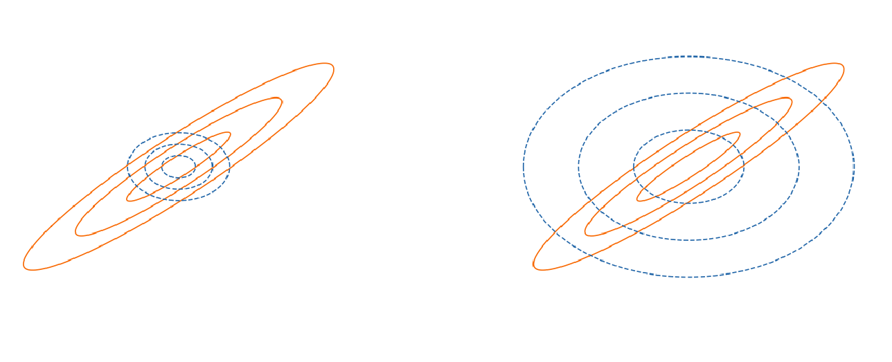
left : backward KL $D_{KL}(q\Vert p)$ (blue is $q$, orange is $p$)
right : forward KL $D_{KL}(p\Vert q)$

ELBO¶

\[ \begin{aligned} Q^* &= \underset{Q\in\mathcal Q}{argmin}~D_{KL}(Q(Z)\Vert P(Z|X)) \\ &= \underset{Q\in\mathcal Q}{argmax}~\mathbb E_{Z\sim Q(Z)}[log(P(X|Z))] - D_{KL}(Q(Z)||P(Z)) \end{aligned} \]

Reparameterization tricks¶

5. Markov Chain Monte Carlo(MCMC)¶

\[ \pi = \pi P \]

where $\pi$ is the stationary state, $P$ is the transition matrix

ergodic : $\exist t\in \mathbb N \rightarrow (P)^t >0$

Metropolis-Hastings Algorithm (MH Algorithm)¶

given proposal distribution $R(x'|x)$ and unnormalized stationary distribution $Q(x)$

accpet rate $\alpha = min\{1, \frac{Q(x')R(x|x')}{Q(x)R(x'|x)}\}$

new transition matrix $col\_standarlize(R \odot \alpha)$

Gibbs Sampling¶

a special case of MH algorithm, with $\alpha_{ij} = 1$

Metropolis Adjusted Langevin Algorithm(MALA)¶

\[ R(x'|x) = \mathcal N(x'|x-\tau \nabla f(x) ;2\tau I) \]

Stochastic Graident Langevin Dynamics (SGLD)¶

\[ \theta_{t+1} = \theta_t - \eta(\nabla log~p(\theta_t) + \frac{N}{n}\sum_{j=1}^n \nabla log p(y_{i_{j}} | \theta_t, x_{i_j})) + \epsilon_t \quad \epsilon_t \sim \mathcal N(0, 2\eta I) \]

where $L(\theta_t)$ is the likelihood

6. Bayesian Deep Learning¶

\[ P(y|x,\theta) = \mathcal N(y;f_\mu(x,\theta_\mu),exp(f_\sigma(x,\theta_\sigma))) \]

\[ \begin{aligned} \hat \theta &= \underset{\theta}{argmin} - lnP(\theta) - \sum_{i=1}^{n}lnP(y_i|x_i,\theta) \\ &= \underset{\theta}{argmin}\lambda ||\theta||^2_2 +\frac{1}{2}\sum_{i=1}^n\left[\frac{1}{\sigma(x_i;\theta_\sigma)^2}||y_i-\mu(x_i;\theta_\mu)||^2 + ln\sigma(x_i;\theta_\sigma)^2\right] \end{aligned} \]

Variational Inference (Bayes by Backprop)¶

\[ \underset{q\in \mathcal Q}{argmin} KL(q||p(\cdot | y)) = \underset{q\in \mathcal Q}{argmax}\mathbb E_{\theta\sim q}[lnP(y|\theta)] - KL(q||p(\cdot)) \]

$p(\cdot)$ is posterior for $\theta$ here

Evidence Lower Bound (ELBO) $$ L(q) = \mathbb E_{\theta\sim q}[lnP(y|\theta)] - KL(q||p(\cdot)) $$

Prediction¶

\[ P(y'|x',X,Y) = \mathbb E_{\theta\sim q}[P(y'|x',\theta)] \]

\[ Var[y'|x',X,Y] = {\color{lightblue}\mathbb E_{\theta\sim q}[Var[y'|x',\theta]]}+{\color{orange}Var[\mathbb E[y'|x',\theta]]} \]

${\color{lightblue}\mathbb E_{\theta\sim q}[Var[y'|x',\theta]]}$ : Aleatoric uncertainty(random)

${\color{orange}Var[\mathbb E_{\theta\sim q}[y'|x',\theta]]}$ : Epistemic uncertainty(knowledge)

Stochastic Weight Averaging-Gaussian(SWAG)¶

\[ \begin{aligned} \mu_{SWA} &= \frac{1}{T}\sum_1^T \theta_i\\ \Sigma_{SWA} &= \frac{1}{T-1}\sum_1^T(\theta_i - \mu_{SWA})(\theta_i-\mu_{SWA})^T \end{aligned} \]

7. Bayesian Optimization¶

Uncertainty Sampling¶

\[ x_t = \underset{x\in D}{argmax}\sigma_{t-1}^2(x) \]

maximizing information gain in homoscedastic noise case
$\underset{t\rightarrow \infin}{lim}~\hat x_t = \underset{\in D}{argmax}~\mu_t(x)$, $f(\hat x )\rightarrow f(x^*)$

Mutual Information $$ F(s) = H(f) - H(f|y_s) = \frac{1}{2}log|I+\sigma^{-2}K_s| \ F(S_T) \ge (1-\frac{1}{e})\underset{S\subseteq D,|S|\le T}{max}~F(S) $$

regret $$ R_T = \sum_{t=1}^T (max_{x\in D}f(x)-f(x_t)) $$ sublinear if $\frac{R_T}{T} \rightarrow 0$

Multi-arm bandit $$ acquisition\uparrow \Longleftrightarrow exploitation\ acquisition\downarrow \Longleftrightarrow exploration $$

Upper Confidence Sampling(UCB)¶

\[ a = \mu_t(x) + \beta \sigma_t(x) \]

Probability of Improvement(PI)¶

\[ a = \Phi\left(\frac{\mu_t(x)-f^*}{\sigma_t(x)}\right) \]

Expected Improvement(EI)¶

\[ a = (\mu_t(x)-f^*)\Phi\left(\frac{\mu_t(x)-f^*}{\sigma_t(x)}\right) + \sigma_t(x)\phi\left(\frac{\mu_t(x)-f^*}{\sigma_t(x)}\right) \]

8. Reinforcement Learning¶

Bellman Theorem $$ V^(x) = max_a(r(x,a) + \gamma\sum_{x'}P(x'|x,a)V^(x')) $$ Hoffeding bound $$ P(|\mu - \frac{1}{n}\sum_{i=1}^n Z_i|>\varepsilon) \leq 2exp(-\frac{2n\varepsilon^2}{C2}) $$

model-based RL

learn Markov Decision Processes, learn $p$ and $r$, e.g gaussian process

model-free RL

learn value function directly

on policy

model has control of the action

off policy

Value Iteration¶

polynomial time, performance depend on the input

guarantee converge to an $\varepsilon$ optimal policy not the exact optimal policy

Policy Iteration¶

guaranteed to monotonically improve the policy

$\boldsymbol \epsilon$ greedy Algorithm¶

model-based

when random number $<\epsilon$ do the random action

R_max algorithm¶

model-based

set reward $R$ and transition probability $P(x^*|x,a)=1$ at first

with probability $1-\sigma$, R_max will reach an $\varepsilon$ - optimal
polynomial time in $|X|, |A|, T,\frac{1}{\varepsilon},log(\frac{1}{\delta})$

Temporal Difference(TD) - Learning¶

model-free

on policy $$ \hat V^\pi (x)\leftarrow (1-\alpha_t)\hat V^\pi (x) + \alpha_t(r+\gamma\hat V^\pi (x')) $$ Theorem $\sum_t\alpha_t=\infin,\sum_t\alpha_t^2 < \infin \Rightarrow P(\hat V^\pi\rightarrow V^\pi) = 1$

Q-Learning¶

model-free: estimate $Q^*$ directly from samples,

off policy $$ \hat Q^* \leftarrow (1-\alpha_t)\hat Q^(x,a) + \alpha_t(r+\gamma \underset{a'}{max}\hat Q^(x',a')) $$ Init: $\hat Q^*(x,a) = \frac{R_{max}}{1-\gamma}\Pi_{t=1}^{T_{init}}(1-\alpha_t)^{-1}$

Theorem $\sum_t\alpha_t=\infin,\sum_t\alpha_t^2 < \infin \Rightarrow P(\hat Q^*\rightarrow Q^*) = 1$

with probability $1-\sigma$, R_max will reach an $\varepsilon$ - optimal
polynomial time in $|X|, |A|, T,\frac{1}{\varepsilon},log(\frac{1}{\delta})$
need decay learning rate to guarantee convergence

DQN¶

\[ L(\theta) = \sum(r + \gamma\underset{a'}{max}Q(x',a';\theta^{old})-Q(x,a;\theta))^2 \]

problem : maximization bias

Double DQN¶

\[ L(\theta) = \sum(r_t + \gamma Q(x_{t+1}, \underset{a'}{argmax}Q'(x,a;\theta');\theta)-Q(x,a;\theta))^2 \]

$\theta' \leftarrow \tau \theta + (1-\tau)\theta'$

Policy Gradient¶

model free $$ J(\theta) = \mathbb E_{\tau\sim \pi_\theta(\tau)}r(\tau) $$

\[ \nabla J(\theta) = \mathbb E_{(x,a)\sim \pi_\theta}[Q(x,a)\nabla log \pi(a|x;\theta)] \]

REINFORCE¶

on policy $$ \begin{aligned} \nabla_{\theta} J(\theta) &= \mathbb E_{\tau\sim p_\theta(\tau)}[\sum_{t=0}^T\gammat(\sum_{t'=t}^T\gammar_t)\nabla_\theta ln\pi_\theta(a_t|x_t)] \ \theta &\leftarrow \theta + \eta_t \nabla_\theta J(\theta) \end{aligned} $$

Policy Search¶

Actor-Critic¶

on policy $$ \begin{aligned} \nabla_{\theta_\pi} J(\theta_\pi) &= \mathbb E_{(x,a)\sim \pi_{\theta_\pi}} [Q_{\theta_Q}(x,a)\nabla_{\theta_\pi}ln\pi_{\theta_\pi}(a|x)] \ \theta_\pi &\leftarrow \theta_\pi + \eta_t \nabla_{\theta_\pi}J(\theta_\pi) \ \theta_Q &\leftarrow \theta_Q - \eta_t(Q_{\theta_Q}(x,a) - r - \gamma Q_{\theta_Q}(x',\pi_{\theta_\pi}(x')))\nabla_{\theta_Q}Q_{\theta_Q}(x,a) \end{aligned} $$

use baseline to reduce variance

Trust- regin policy optimization (TRPO)¶

on policy

$$

Proximal Policy Optimization (PPO)¶

on policy $$ L_{\theta_k}(\theta_k) = \mathbb E{\tau \sim \pi_k}\sum_{t=0}^\infin[\frac{\pi_\theta(a_|x)}{\pi_{\theta_k}(a|x)}(r + \gamma Q^{{\pi_{\theta_k}}(x',a)-Q}(x,a))] \ \theta_k \leftarrow \theta_k - \eta_t \nabla_{\theta_k}L_{ \theta_k}(\theta_k) $$}

Deep Deterministic Policy Gradients(DDPG)¶

off policy

randomly add noise the ensure sufficient exploration $$ \begin{aligned} \theta_Q &\leftarrow \theta_Q - \eta \nabla_{\theta_Q} \mathbb E_{\tau\sim\pi_{\theta_\pi}}[(Q_{\theta_Q}(x, a)-(r + \gamma Q_{\theta_Q^{{old}}(x',\pi_{\theta_\pi}(x')))^2] \ \theta_\pi &\leftarrow \theta_\pi + \eta \nabla_{\theta_\pi} \mathbb E_{\tau\sim\pi_{\theta_\pi}}[Q_{\theta_Q}(x,\pi_{\theta_\pi}(x))] \ \theta_Q^{old} &\leftarrow (1-\rho)\theta_Q^{old} + \rho \theta_Q \ \theta_\pi^{old} &\leftarrow(1-\rho)\theta_\pi^{old} + \rho \theta_\pi}

\end{aligned} $$

Soft Actor Critic(SAC)¶